A Cluster-Analytic Approach to Constraint Typologies and Technical Efficiency among Maize Farmers in Himachal Pradesh

1. Introduction

Maize (Zea mays L.) is one of the world’s three dominant cereals, alongside rice and wheat, and is an essential component of global agri-food systems (Erenstein et al., 2022; Ranum et al., 2014). Beyond its role as a staple food, maize increasingly drives the food–feed–fuel nexus, supplying raw materials for livestock feed, starch-based industries, and emerging bio-ethanol markets (OECD & FAO, 2025; USDA-FAS, 2025). India is the world’s sixth-largest maize producer, cultivating about 9.9 million hectares and contributing nearly 3 percent of global output. However, national yields average only 3.1 t/ha, far below the global mean of 5.8 t/ha (Erenstein et al., 2022; Economics, Statistics, and Evaluation Division, 2023).

Maize production conditions differ substantially across India’s agro-ecological regions. In the irrigated plains of the Indo-Gangetic, maize cultivation operates within a relatively input-intensive production environment, supported by extensive irrigation infrastructure, greater mechanization, and stronger market linkages (Jat et al., 2025). By contrast, low-hill production systems are predominantly rain-fed and characterized by small, fragmented landholdings, with limited mechanization and increasing reliance on household labor. Evidence from South Asia shows that mechanization intensity and technology adoption are strongly conditioned by farm size and topography (Aryal et al., 2021). These structural differences suggest that the drivers of maize productivity and technical efficiency vary across agro-ecological contexts, highlighting the importance of context-specific analysis in low-hill production systems.

In India, maize holds particular significance in Himachal Pradesh, where geoclimatic conditions favor its cultivation in the low- and mid-hill agroecological zones. Maize occupies nearly 300 thousand hectares, around one-fifth of the state’s gross cropped area, and is predominantly grown as a rain-fed kharif crop on small and highly fragmented holdings (Department of Economics & Statistics, 2022; ICAR–Indian Institute of Maize Research, 2022).These structural characteristics shape the maize cultivation environment in the state, where farmers face both climatic risks and persistent structural and institutional constraints.

As a predominantly rain-fed crop, maize production is particularly sensitive to climatic variability. Recent evidence documents rising rainfall variability, extended dry periods, and irregular monsoon patterns across the state, increasing yield variability and production risk (KC et al., 2022; S. Kumar & Singh, 2023; Srivastava et al., 2021). In addition to rainfall variability, climate change is also altering pest and disease pressure in maize-based farming systems. Shifting temperature and humidity conditions have increased the incidence of insect pests and plant diseases, constraining crop productivity (Ma et al., 2024). Recent field evidence from Himachal Pradesh documents measurable pest-related yield losses under local agro-climatic conditions, highlighting the economic significance of biotic constraints in maize cultivation (Kharwal et al., 2025). These pressures contribute to yield reductions and often require additional pest-management inputs, thereby raising production costs and potentially reducing technical efficiency (Chatterjee et al., 2023). Such interactions underscore the importance of examining pest and disease pressure as a distinct production constraint within location-specific farming systems.

Furthermore, socio-economic and institutional constraints, combined with agronomic risks, place additional burdens on smallholder farmers. Rising input costs and persistently low maize returns compress farm margins, weakening the economic viability of maize cultivation and limiting reinvestment capacity. Within this constrained economic environment, limited access to quality agricultural inputs, uneven coverage of public provisioning systems, and persistent financial barriers further restrict farmers’ ability to adopt improved production practices (A. N. Thakur, 2024). Labor scarcity compounds these challenges. As the availability of rural labor declines, dependence on machinery increases; however, financial and structural constraints continue to slow the adoption of mechanization (Aryal et al., 2021; Rajkhowa & Kubik, 2021). In addition, the prevalence of small and fragmented landholdings further reduces the economic feasibility of mechanization, particularly in low-hill production systems (Roy et al., 2022). Beyond economic and structural barriers, ecological pressures further compound production risks. Wild-animal incursions, particularly by monkeys and wild boars, cause frequent and severe crop losses in low- and mid-hill villages (R. K. Thakur et al., 2022).

Even when farmers adopt improved inputs, productivity outcomes often remain unstable because climatic, biological, and socio-economic pressures interact to create complex and overlapping production environments (Kumari & Sharma, 2018; S. Kumar & Singh, 2023; P. Kumar et al., 2025; Negi et al., 2012). As a result, farmers operate within multidimensional constraint systems in which the combined effects of multiple barriers shape both yield performance and technical efficiency (KC et al., 2022). Because production constraints often operate jointly, assessing them in isolation may overlook important variations in productivity and technical efficiency across farms.  In the present study, fifteen farmer-ranked production constraints are analysed and subsequently grouped into six empirically derived constraint typologies using hierarchical clustering techniques. Rather than treating individual barriers independently, this approach identifies distinct multidimensional constraint environments that shape farm performance. These typologies provide the analytical basis for examining heterogeneity in technical efficiency and maize output.

This typology-based perspective is consistent with emerging global evidence showing that technical efficiency improves when production, information, and risk constraints are addressed collectively. This is demonstrated by integrated water–nutrient management in the North China Plain, which increased yields by 1.6 percent annually while reducing greenhouse-gas intensity by 17 percent (Wang et al., 2023). A randomized controlled trial in Kenya showed that a bundled package of credit, high-quality inputs, training, and insurance increased maize yields by about 26 percent (Deutschmann et al., 2025). These examples illustrate the importance of adopting a multi-constraint view of productivity shortfalls rather than evaluating individual constraints in isolation. Earlier Indian work combining analysis with frontier modeling, notably Banerjee et al. (2014) for maize systems, demonstrated that efficiency losses arise from interactions among institutional and socio-economic barriers. Similar multivariate approaches in dairy systems (Baral & Bardhan, 2016) further reinforce the role of structural heterogeneity in shaping farm performance. However, rigorous empirical evidence on how multidimensional constraints influence agricultural efficiency remains limited.

Despite extensive literature on climate risks, pest dynamics, and socio-economic barriers, two critical gaps persist. First, there is an empirical understanding of how farmer-perceived constraints cluster together where risks are highly localized and interdependent. Second, few studies have examined how these constraint typologies relate to technical efficiency and output performance. No previous work has integrated ranked-constraint data with both hierarchical clustering and stochastic frontier analysis to explain performance heterogeneity among maize growers in Himachal Pradesh.  Given these gaps, the present study examines how different combinations of farmer-perceived production constraints influence technical efficiency and maize output in the low-hill zone of Himachal Pradesh. Using ranked constraint data from maize-growing households, the analysis applies the Salama–Quade weighted rank correlation and hierarchical clustering to identify empirically grounded constraint typologies. These typologies are subsequently linked to efficiency estimates from Stochastic Frontier Analysis (SFA) and to output regressions estimated using ordinary least squares. By integrating ranked-constraint data with frontier modelling, the study provides new empirical evidence on how multidimensional constraint environments shape performance heterogeneity in smallholder maize systems. The paper is organized as follows: Section 2 presents the data and variables; Section 3 explains the methods used in the analysis; Section 4 reports the results; Section 5 discusses the findings; and Section 6 concludes the study.

2. Data and Variables

Primary data were collected during 2023–24 using a multistage cluster sampling design and a structured questionnaire. At the first stage, three districts, Kangra, Mandi, and Hamirpur, were purposively selected as they together account for nearly 48% of the maize-harvested area in Himachal Pradesh. In the second stage, nine major maize-growing blocks were identified, namely Karsog, Gohar, and Sadar (Mandi); Bamson, Bhoranj, and Hamirpur (Hamirpur); and Nurpur, Fatehpur, and Dehra (Kangra). At the third stage, four panchayats were selected from each block, and one village was chosen from each selected panchayat, yielding a total of 36 panchayats and 36 corresponding villages. Finally, 12 farm households were randomly selected from each village, yielding a total sample of 432 maize-producing households. This sampling process ensured the use of diverse maize-growing conditions across the study area. The findings are therefore most directly applicable to districts with similar agro-climatic and production characteristics, and may not fully capture conditions prevailing in areas where maize plays a relatively minor role.

As part of the questionnaire, farmers were asked to rank 15 production constraints affecting maize cultivation from 1 (most severe) to 15 (least severe). The constraint items included high input costs, low maize returns, weather and climate variability, wild animal crop damage, pest and disease pressure, lack of financial assistance, labor shortage, limited access to improved seed, declining soil fertility, inadequate research and extension support, fragmented landholdings, under-mechanized agriculture, crop insurance challenges, irrigation access constraints, and land tenure issues. These constraints were identified based on prior literature, regional agronomic conditions, and pre-survey consultations with farmers and extension officials to ensure contextual relevance.

The socio-economic profile and institutional characteristics of the sampled households are summarized in Table A1. The majority of sampled households fall within the marginal and small farm categories, with approximately 80 percent cultivating less than two hectares. Education levels were limited, with nearly one-third of respondents being illiterate. Although adoption of improved maize seed was relatively high, access to institutional support remained limited. Fewer than one-fifth of sampled households possessed a Kisan Credit Card, and awareness of the minimum support price was low. Crop insurance coverage was negligible. Around half of the households reported receiving technical advice from extension agents or other sources, but participation in soil health card schemes and formal training programs remained minimal. For the efficiency and output estimations, the key production variables included total maize output (kg per household), operated land area (hectares), seed use (kg), fertilizer (kg), labor (hours), machinery use (hours), and pesticide expenditure (₹) during the 2023–24 kharif season. Fertilizer denotes the combined quantity of chemical fertilizer and farmyard manure applied by the household. Table 1 reports summary statistics of maize output and production inputs. Average maize output was 928 kg per household, with substantial dispersion across farms, reflecting heterogeneity in production scale. Operated land averaged 1.07 hectares, consistent with the smallholder structure of maize cultivation in the study area. Considerable variation is also observed in fertilizer use and labor input, suggesting differences in input intensity across farms. Machinery use and pesticide expenditure display high dispersion relative to their means, indicating uneven adoption of mechanization and crop protection practices. Such variability in input use supports the application of a stochastic frontier framework to assess efficiency differentials.

Table 1. Descriptive Statistics for Input–Output Variables.

Source: Author’s calculations.

3. Methods

3.1. Clustering of Ranked Production Constraints

3.1.1. Salama–Quade Similarity

The units of analysis in this study are maize-growing farm households characterized by their ranked production constraints. These rankings were used to group farmers based on how they prioritized production constraints. The focus is on identifying heterogeneity in production constraints across farmers rather than relying on average rankings. The clusters reported in the results are derived from similarity patterns in these fifteen ranked constraint items and do not represent predefined categories. To quantify the similarity of farmers’ ranked constraints, the Salama–Quade (SQ) weighted rank correlation was computed for every pair of farmers. The SQ correlation is appropriate for ordinal data because it assigns greater weight to higher-ranked items, reflecting the fact that higher-ranked constraints have greater informational value than lower-ranked ones (Salama & Quade, 1982). Similarity between farmers’ ranked constraint profiles was measured using the Salama–Quade (SQ) weighted rank coefficient. For a pair of farmers  and , define the pair-specific weight for constraint  as:

where denotes the number of farmers and  the number of constraints and  denote the rank assigned by the farmer () to constraint (). After data cleaning, all farmers provided complete rankings, so is constant across all farmer pairs. which assigns greater influence to constraints that receive lower ranks (i.e., are perceived as more severe). The Salama–Quade similarity coefficient between farmers  and  is defined as:

In equation (2),  indexes rank positions from 1 to . The numerator represents the weighted squared difference in ranks across constraints. The denominator is a normalising constant that depends only on  and ensures comparability across farmer pairs.

3.1.2. Dissimilarity Transformation

The SQ rank-correlation matrix was converted into a farmer-to-farmer dissimilarity matrix for use as input to the clustering analysis. Dissimilarity was computed using a standard linear transformation:

This transformation allows farmers with similar constraint rankings to be grouped together in the clustering stage, where  denotes the dissimilarity between farmers and , and ) is the Salama–Quade correlation. The resulting  dissimilarity matrix captures the pairwise distance between all farmers based on the weighted differences in their ranked constraints.

3.1.3. Agglomerative Hierarchical Clustering

After computing the rank-based dissimilarity matrix, farmers were grouped using agglomerative hierarchical clustering (AHC) with the complete-linkage criterion (Johnson, 1967). AHC was preferred because it allows farmer groups to emerge directly from the dissimilarity structure without pre-specifying the number of clusters (Brentari et al., 2016; Fonseca, 2013; Kaufman & Rousseeuw, 2009). Complete linkage was used to emphasize compact, well-separated clusters. Under the complete linkage criteria, the distance between two clusters and  is defined as the maximum pairwise dissimilarity between any member of the cluster and any member of :

where  represents the dissimilarity between farmers and . AHC has been widely applied in social science and agricultural research to develop interpretable farmer typologies based on multidimensional data (Etumnu & Gray, 2020; Rasool & Abler, 2023).

3.1.4. Silhouette Index

In the present study, the optimal number of clusters was assessed using the silhouette index, which measures how well each observation is assigned to its cluster relative to other clusters (Kaufman & Rousseeuw, 2009). Let denote the cluster containing the farmer , and let denote set cardinality. Define

For farmer , the silhouette value is defined as:

where denotes the average dissimilarity of farmer with all other farmers in the same cluster, and is the lowest average dissimilarity of farmer to any other cluster of which is not a member.

In this study, the average silhouette width (ASW) was computed for alternative solutions with 2 to 20 clusters using the SQ-based dissimilarity matrix. The average silhouette width (ASW) is:

The final number of clusters was selected based on the highest ASW, with support from a visual inspection of the dendrogram. The corresponding silhouette values for the potential cluster solutions are reported in the results section.

3.1.5. Cluster Stability (Bootstrap Jaccard Coefficient)

To assess whether the identified farmer clusters were robust to sampling variation, cluster stability was evaluated using bootstrap resampling. Cluster stability is important because bootstrap-based evaluation provides a measure of how consistently each cluster appears across repeated samples (Hennig, 2007). The Jaccard coefficient is defined as:

where is the number of farmers retained in both the original and bootstrap-derived clusters, and is the total number of unique farmers belonging to either cluster. Jaccard values range from 0 to 1, with higher values indicating stronger stability. Following established practice, higher Jaccard values were interpreted as indicating greater cluster stability, while lower values were treated as reflecting weaker or less consistent groupings (Hennig, 2007). In this study, 200 bootstrap replications were performed using the cluster boot function in the fpc package in R. The Jaccard stability values for all six clusters are reported in the results section.

3.2. Plackett–Luce Model for Aggregate Constraint Ranking

Alongside the cluster-based analysis of ranked constraints, we also estimated a Plackett–Luce (PL) model to obtain an overall ordering of production constraints across all farmers. While clustering captures heterogeneity in how constraints are prioritized, the PL model provides a summary measure of each constraint's relative severity at the aggregate level. In this application, each of the fifteen maize production constraints was treated as an item, and the estimated worth parameters reflect their relative importance as perceived by farmers. The PL model was estimated using the Plackett-Luce package in R, which is designed for analyzing full and partial ranking data (Turner et al., 2020). The resulting worth parameters were rescaled to sum to one and are reported along with quasi-standard errors to indicate the precision of the estimates. While the Salama–Quade correlations and agglomerative hierarchical clustering capture heterogeneity in constraint patterns across farmers, the PL model provides a complementary system-level ranking of constraints for the sample as a whole.

3.3. Stochastic Frontier Model

Following the identification of constraint-based farmer clusters, their association with technical efficiency (TE) and maize output was analyzed using a combination of Stochastic Frontier Analysis (SFA) and Ordinary Least Squares (OLS) output models. This sequential framework allows us to distinguish how constraint typologies influence (i) production efficiency and (ii) observed output levels, while controlling for farm, technology, and demographic characteristics.

Efficiency was estimated using a stochastic frontier framework rather than a deterministic Data Envelopment Analysis (DEA) approach. As a deterministic frontier method, DEA attributes deviations from the frontier to inefficiency (Charnes et al., 1978). In contrast, stochastic frontier analysis (SFA) decomposes the composite error into a symmetric noise term and a non-negative inefficiency term, thereby accounting for random shocks and measurement error (Coelli et al., 2005). Agricultural output is subject to stochastic influences such as weather variability and measurement error (Battese, 1992; Bravo-Ureta & Pinheiro, 1993). The stochastic frontier model separates statistical noise from inefficiency within a parametric likelihood framework (Aigner et al., 1977; Kumbhakar et al., 2021; Meeusen & van Den Broeck, 1977).

The stochastic frontier model is specified as:

where denotes the maize output of the farm , is a vector of production inputs including landholding (ha), seed use (kg), fertilizer use (kg), labour (hours), machinery use (hours), and pesticide expenditure (₹), represents statistical noise, and  captures technical inefficiency (Aigner et al., 1977). This specification allows deviations from the frontier to reflect both random shocks and inefficiency within a parametric likelihood framework (Kumbhakar et al., 2021).

The production function was specified in both Cobb–Douglas and Translog forms. The Cobb–Douglas specification is written as:

where denotes the -th input for farm , and is the number of inputs included in the production function. The Translog specification extends this as:

The Translog provides a flexible second-order approximation to an arbitrary production function, whereas the Cobb–Douglas is a restricted nested specification (Christensen et al., 1973). To assess the appropriate functional form, a likelihood ratio (LR) test was conducted:

where  represents the restricted Cobb–Douglas model and denotes the unrestricted Translog specification. The statistic follows a chi-square distribution with degrees of freedom equal to the number of imposed restrictions.

Both specifications were estimated using maximum likelihood methods consistent with standard stochastic frontier practice (Greene, 2003; Kumbhakar et al., 2021).

Alternative distributional assumptions were considered for the inefficiency term. The half-normal specification assumes that inefficiency follows a one-sided normal distribution with zero mean, whereas the truncated-normal specification allows a non-zero mean and greater flexibility (Aigner et al., 1977; Stevenson, 1980). Because efficiency estimates may be sensitive to the assumed distribution, both specifications were estimated and compared using information criteria consistent with standard stochastic frontier practice (Kumbhakar et al., 2021). Model selection was guided by likelihood-ratio tests for nested specifications and by information criteria, including the Akaike Information Criterion (AIC) and the Bayesian Information Criterion (BIC; Akaike, 1974; Schwarz, 1978), with preference given to the more parsimonious specification when competing models provided comparable fit (Burnham & Anderson, 2004).

Technical inefficiency was modeled within the stochastic frontier following the one-step approach of Battese and Coelli (1995). In this framework, the non-negative inefficiency term is specified as:

where  is a vector of variables influencing inefficiency, is a parameter vector, and follows a normal distribution truncated at zero. The vector includes farm, household characteristics, as well as cluster indicators entered as fixed effects in the inefficiency component. Cluster indicators are incorporated in the inefficiency equation rather than the production frontier to allow systematic variation in technical inefficiency across constraint typologies while maintaining a common production function for all farms. All parameters were estimated jointly by maximum likelihood.

Technical efficiency scores were obtained from the estimated frontier using the conditional expectation approach of Jondrow et al. (1982). In this method, inefficiency is estimated as , where is the composed error term. Farm-level technical efficiency is then calculated as:

with values bounded between 0 and 1.

3.4. OLS Output Models

In addition to efficiency outcomes, cluster differences in production levels were examined using the logarithm of total maize output as the dependent variable:

where  is a binary indicator equal to 1 if the household  belongs to a cluster  (for ) and 0 otherwise, with Cluster 1 serving as the reference category. Wi denotes additional covariates introduced sequentially across specifications. These OLS models capture reduced-form output differentials associated with constraint typologies without imposing the stochastic frontier structure. All econometric analyses were implemented in R (R Core Team, 2025).

4. Result

4.1. Cluster Identification and Validation

Agglomerative hierarchical clustering applied to the SQ-based dissimilarity matrix resulted in a six-cluster solution. The average silhouette width (ASW) was 0.43, corresponding to a moderate level of cluster structure (Figure 1). Although this reflects only moderate separation, the distribution of silhouette values provides further insight into the structure of the solution. Approximately 91% of observations exhibit positive silhouette scores, and the median silhouette width is 0.50 (Figure 2), suggesting that most farmers are more similar to members of their assigned cluster than to those in neighboring groups. Further evidence of internal coherence is provided by dispersion diagnostics. As shown in Table 2, the mean within-cluster dissimilarity (0.0042) is substantially lower than the mean between-cluster dissimilarity (0.0114), yielding an overall within-to-between ratio of 0.37. This pattern is observed across clusters and indicates that farmers grouped together share relatively similar constraint profiles compared with those in other clusters. To assess sensitivity to methodological choices, the clustering procedure was repeated using alternative linkage criteria. The resulting partitions show strong agreement with the complete-linkage solution, with adjusted Rand indices of 0.75 (average linkage) and 0.78 (Ward D2; Table A2). These results suggest that the six-cluster structure is not driven by the specific linkage rule employed. The dendrogram structure was preserved across resamples, confirming that the six-cluster solution reflects an underlying and reproducible segmentation of farmers based on constraint patterns (Figure 3).

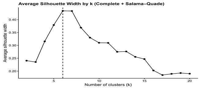
Figure 1. Average silhouette width (ASW) across alternative cluster solutions (k = 2–20).

Note: Clustering performed using agglomerative hierarchical clustering with complete linkage on the rank-based dissimilarity matrix (N = 432). Vertical line indicates the six-cluster solution.

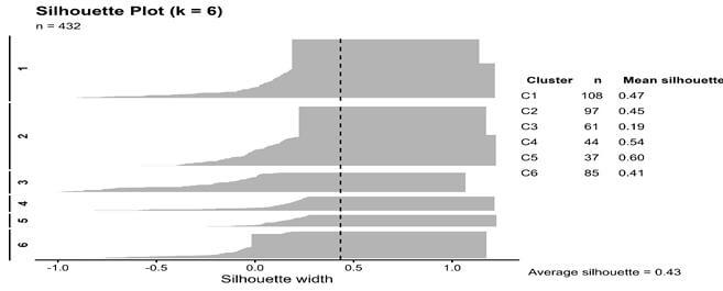
Figure 2. Silhouette widths for the six-cluster solution.

Note: Average silhouette width (ASW = 0.43) indicates moderate separation and internal consistency across clusters.

Table 2. Within- and Between-Cluster Salama–Quade Dissimilarity (k = 6).

Note: Dissimilarity values are based on the Salama–Quade rank-based distance metric. Ratios below 1 indicate that within-cluster dissimilarity is substantially lower than between-cluster dissimilarity, supporting internal coherence of the identified groups.

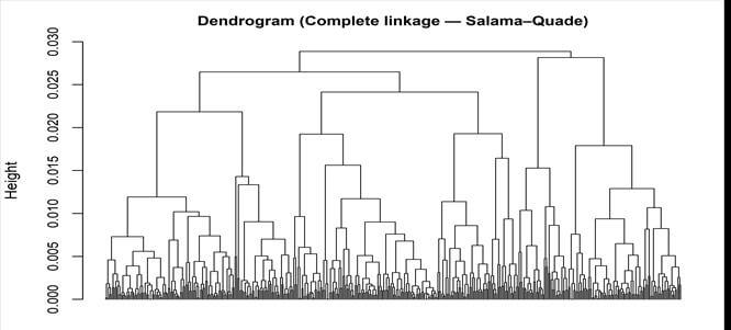
Figure 3. Complete-linkage dendrogram based on rank-dissimilarity matrix.

Note: Clustering performed using agglomerative hierarchical clustering with complete linkage on the rank-based dissimilarity matrix (N = 432). Vertical line indicates the six-cluster solution.

Table 3 presents the Jaccard similarity coefficients, which indicate variation in stability across clusters. Cluster C5 shows the highest stability (0.80), followed closely by C1 (0.80) and C6 (0.76). Cluster C2 exhibits moderate stability (0.74), while C4 (0.67) and C3 (0.65) display comparatively lower, though acceptable, stability levels. Across bootstrap samples, recovered clusters consistently outnumbered dissolved clusters, indicating that the six-cluster structure is reproducible. Overall, the bootstrap results support the robustness of the identified segmentation. The dendrogram structure was preserved across resamples, confirming that the six-cluster solution reflects an underlying and reproducible segmentation of farmers based on constraint patterns.

Table 3. Cluster Stability Measures (Jaccard, Dissolved, Recovered).

Note: Stability based on 200 bootstrap replications; Jaccard = mean similarity between original and resampled clusters. Stability classification follows Hennig (2007).

4.2. Cluster Profiles and Spatial Distribution

The six clusters identified through hierarchical clustering exhibit distinct patterns in production constraint rankings (Figure 4). The six clusters are labelled as follows: C1 (Climate Variability), C2 (Wildlife Damage), C3 (Seed Access), C4 (Land Fragmentation), C5 (Mechanization-Constraint Salient), and C6 (Pest and Disease Pressure). These differences are not only statistical but also associated with variations in farm size, institutional participation, and district-level distribution. Evidence from Table 4, Figure 5, and Figure 6 shows that each cluster reflects a distinct maize production setting. The clusters are therefore discussed below by linking their constraint profiles with socio-economic characteristics and spatial concentration. Cluster C1 is characterized by the prominence of weather and climate variability (mean rank 1.27), followed by declining soil fertility (3.07) and low returns (4.69). The ranking pattern points to environmental instability as the central concern within this group, distinguishing it from clusters shaped primarily by land structure or input access. Most farmers in C1 operate marginal holdings (64%), with a further 22% classified as small farmers, limiting their ability to buffer rainfall fluctuations through scale advantages. Improved seed adoption is moderate (57%), and participation in formal mechanisms such as Kisan Credit Cards (16%) and technical advice (43%) remains modest. Crop insurance coverage is extremely low (3.7%), and with marginal and small holdings dominating this cluster, formal financial protection against climatic shocks remains limited. The cluster is heavily concentrated in Mandi (65%), where exposure to rainfall variability during the kharif season increases production uncertainty. In such settings, climatic risk interacts with small farm size and weak insurance coverage, reinforcing vulnerability to weather shocks.

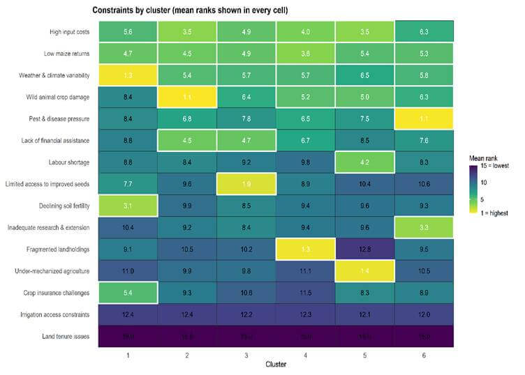
Figure 4. Cluster-wise rank profiles of constraints (C1–C6).

Note: Lower ranks indicate more severe constraints. C1–C6 correspond to the six identified constraint typologies.

Table 4. Farmers’ characteristics by cluster (categorical variables; χ² tests with Holm-adjusted p-values).

 

Table 4. Cont.

Note: Values denote the number of farmers within each category, with percentages shown in parentheses. P-values are adjusted using the Holm method for multiple comparisons.

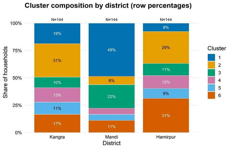
Figure 5. District-wise distribution of constraint clusters (C1–C6).

Note: Each bar represents the proportion of farmers in each constraint cluster across Kangra, Mandi, and Hamirpur districts.

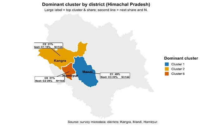
Figure 6. Dominant constraint cluster by district in Himachal Pradesh.

Cluster C2 is dominated by wild-animal crop damage (mean rank 1.08), followed by high input costs (3.51) and constraints in accessing financial support (4.45). This profile reflects a production context in which exposure to wildlife damage, rather than land structure or input scarcity, shapes perceptions of constraint. Farm characteristics indicate relatively active engagement in production. Improved seed adoption (89%) and KCC participation (29%) indicate that farmers in this cluster have access to institutional support. However, formal financial access remains limited for a substantial share of farmers. This combination suggests that crop losses from wildlife occur despite moderate technological and institutional participation. The cluster is concentrated in Kangra (45%) and Hamirpur (43%), with limited presence in Mandi (11%). Reported damage largely involves stray cattle and monkeys rather than forest wildlife, pointing to recurring crop disturbance in village peripheries. Under such conditions, wildlife exposure remains a persistent risk that undermines output stability even where input use is relatively high.

Cluster C3 is characterized by restricted access to improved seed (mean rank 1.85), followed by financial constraints (4.67) and low returns (4.89). This profile identifies input access as the central constraint within this group. Improved seed use is low: 87% of farmers in C3 do not use improved varieties, representing the highest non-adoption rate across clusters. Credit participation is limited, with only 9.8% holding a Kisan Credit Card, and MSP awareness is similarly low. Landholdings are largely marginal (67%) or small (25%), which may restrict purchasing capacity and regular access to quality seed. C3 is most prevalent in Mandi (51%), with smaller shares in Hamirpur (26%) and Kangra (23%). In this context, limited seed adoption appears to be closely linked to farm size and restricted institutional access rather than to environmental conditions. The cluster farm-level conditions in which access to improved seed technology remains the primary constraint. C4 is defined by very small landholdings. Nearly all households (98%) operate marginal farms, making this the most land-constrained group in the sample. Land fragmentation receives the lowest mean rank (1.32), followed by low returns (3.59) and rising input costs (3.95), indicating that operational scale, rather than climatic or input-access factors, defines this typology. Although participation in improved seed use and technical advice is present, the extremely small land base limits opportunities for mechanization and scale efficiency. In this cluster, production capacity is shaped primarily by farm size rather than by access to technology or institutions. C4 is largely present in Kangra (43%) and Hamirpur (39%), with a smaller share in Mandi (18%). Where marginal holdings dominate, limited operational scale continues to constrain productivity over time. Cluster C5 is characterized by mechanization as the most salient constraint (mean rank 1.43), followed by input costs (3.51) and labor shortages (4.22), while wildlife damage ranks lower (5.0). The ranking pattern points to operational scale rather than basic resource scarcity as the defining feature of this group. Farm characteristics indicate comparatively greater production capacity. A substantial share of farmers operate small (41%) and semi-medium holdings (43%), and improved seed adoption is widespread (92%). Participation in technical advice is also high (78%), indicating active engagement with formal agricultural services. In this farm structure, mechanization becomes a scale-related requirement, particularly where timely field operations and labor management become more important as farm size increases. C5 is distributed across Kangra (43%), Hamirpur (35%), and Mandi (22%), suggesting that the pattern is linked to farm structure rather than district-specific conditions. Therefore, mechanization appears as a constraint associated with scale-intensive maize production.

Cluster C6 is characterized by the prominence of pest and disease pressure (mean rank 1.12), followed by research and extension gaps (3.33) and low returns (5.27). The ranking pattern identifies biological stress as the central constraint within this group. The cluster is concentrated in Hamirpur (53%), with smaller shares in Kangra (28%) and Mandi (19%), indicating localized exposure to pest-related risks. Although improved seed use is widespread (95%), recurrent pest incidence appears to undermine yield stability. The simultaneous prominence of low returns suggests that production outcomes are influenced less by input availability and more by biological vulnerability. C6 represents a maize production environment in which pest pressure remains the dominant factor influencing farm performance.

This pattern is consistent with the Plackett–Luce worth estimates, where low returns (15.5%), climate risk (15.3%), input costs (13.7%), wild-animal damage (10.9%), and pest pressure (8.6%) together account for more than 64% of total constraint severity in the sample (Figure 7). These results indicate that while certain pressures are widely shared across farmers, the cluster analysis reveals how different constraints become locally dominant depending on farm structure and district context.

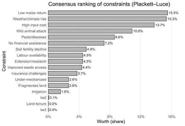
Figure 7. Plackett–Luce worth estimates for ranked production constraints.

Note: A higher value indicates a greater probability that a constraint will be ranked as most severe.

4.3. Model Selection and Robustness

We first compare the Cobb–Douglas and translog specifications using likelihood ratio (LR) tests. Since the Cobb–Douglas model is a restricted version of the translog specification, the LR test evaluates whether the additional squared and interaction terms are jointly significant. As reported in Table A3, the LR statistics reject the restrictions implied by the Cobb–Douglas form under both distributional assumptions, indicating that the translog model provides a statistically better fit in a nested comparison. However, once model complexity is penalized through information criteria, the incremental improvement in fit becomes negligible. The translog specification substantially increases the number of estimated parameters, while yielding only a marginal gain in log-likelihood. The information criteria reported in Table A4 show only minor differences in AIC values across specifications, and the BIC does not provide clear support for the more parameter-intensive translog model. Given the limited increase in log-likelihood relative to the substantial rise in the number of estimated parameters, the simpler Cobb–Douglas specification offers a more stable and interpretable representation of production technology in this sample. This choice is consistent with the principle of parsimony in model selection, which favors the simplest specification that adequately captures the data-generating process (Burnham & Anderson, 2004).

We also compare half-normal and truncated-normal distributions for the inefficiency term. The truncated-normal specification demonstrates a slightly better fit and stable convergence within the one-step framework and is therefore adopted as the preferred distributional assumption. Finally, efficiency estimates are highly consistent across alternative specifications. As shown in Table A5, correlations between efficiency scores exceed 0.95, while Table A6 indicates that mean efficiency levels vary only marginally across models. This stability suggests that the study’s substantive conclusions are not sensitive to the choice of functional form or the inefficiency distribution. Accordingly, the Cobb–Douglas truncated-normal model is selected as the preferred specification, with alternative models used for robustness analyses.

Table 5 presents the estimates of the alternative stochastic frontier specifications. The estimated gamma (γ = 0.953) suggests that a substantial share of the unexplained variation in maize output is attributable to technical inefficiency rather than random shocks. The sum of the input elasticities is approximately 0.48, indicating decreasing returns to scale. This implies that a proportional increase in all inputs would lead to a less-than-proportional increase in total maize output. The estimated parameters for the production inputs are statistically significant, except for fertilizer. Among the production inputs, labor has the largest elasticity (0.172), indicating that labor plays the most prominent role in maize production. A 1% increase in labor is associated with a 0.17% increase in output, highlighting the labor-intensive nature of cultivation practices in the study region.

Table 5. Stochastic Production Frontier Estimates (One-Step CD_TN Model).

Note: Dependent variable is ln(output). The model is estimated using a truncated-normal stochastic frontier specification. Standard errors are in parentheses.

^*** p < 0.01, ^** p < 0.05, ^* p < 0.10.

Land and seeds are also positively associated with output, with elasticities of 0.118, suggesting that expanding cultivated area and improving seed use increase production. Machinery and pesticides have smaller effects, whereas fertilizer is not statistically significant. Maize production remains labor-intensive, with substantial variation in efficiency across farmers.

4.4 Technical Inefficiency and Cluster Effects

The cluster fixed effects in the inefficiency component reveal meaningful differences across typologies (Table 6). In the baseline specification (M1), C5 is associated with substantially lower inefficiency relative to the reference group (C1), and this relationship remains stable across subsequent specifications. In the final specification (M4), the estimated coefficient increases in absolute value and remains statistically significant, indicating that Cluster 5’s efficiency advantage persists after accounting for farm structure, technology adoption, household characteristics, and regional heterogeneity. C6 is associated with a negative, statistically significant coefficient in intermediate specifications; however, this association becomes statistically insignificant once the full set of covariates is included. C2, C3, and C4 do not differ statistically from the reference group in the final model.

Table 6. Cluster-Specific and Determinants of Inefficiency (One-Step SFA Model).

Note: C1 is the reference category. Marginal holding (< 1 ha) is the base category. District Kangra is the reference district.

^*** p < 0.01, ^** p < 0.05, ^* p < 0.10.

In the fully specified model (M4), landholding size is negatively associated with inefficiency. Farms of 2 hectares or more show a substantial reduction in inefficiency (−0.967), while holdings of 1–2 hectares also exhibit lower inefficiency (−0.478) relative to marginal farms. This pattern indicates that a larger operational scale is associated with lower inefficiency. The use of improved seed is likewise associated with lower inefficiency (−0.641), suggesting that adoption of enhanced varieties contributes to improved production outcomes. Household size is also negatively associated with inefficiency, suggesting that farms with greater family labor availability tend to perform better. In contrast, institutional variables and demographic characteristics such as KCC access, MSP awareness, technical advice, age, and literacy do not show statistically significant effects in the fully specified model. Regional differences remain pronounced. Farmers in Mandi district exhibit significantly lower inefficiency (−0.997), whereas those in Hamirpur display higher inefficiency (0.476) relative to the reference district. The results indicate that efficiency differences across clusters are largely explained by farm structure and regional characteristics, with C5 remaining statistically distinct in the fully specified model.

Table 7 and Figure 8 present the cluster-wise mean technical efficiency scores based on the final one-step CD–TN model. The overall mean efficiency is 0.604, indicating that maize farmers operate, on average, at about 60% of the potential frontier output given existing inputs. C5 records the highest mean efficiency (0.857; 95% CI: 0.825–0.888), clearly above the sample average. This level is substantially higher than the overall sample mean (0.604), indicating a pronounced efficiency differential. In contrast, Cluster 4 (0.52) and Cluster 6 (0.538) show comparatively lower efficiency levels, while Clusters 1–3 are concentrated around 0.60–0.61. These descriptive differences align with the regression results, where Cluster 5 remains the only group with a statistically distinct inefficiency effect in the fully specified model.

Table 7. Mean Technical Efficiency by Cluster (One-Step CD_TN Model).

Note: Technical efficiency scores are derived from the preferred one-step truncated-normal stochastic frontier model. Values are rounded to 2 decimal places and represent the mean efficiency by cluster, with 95 confidence intervals.

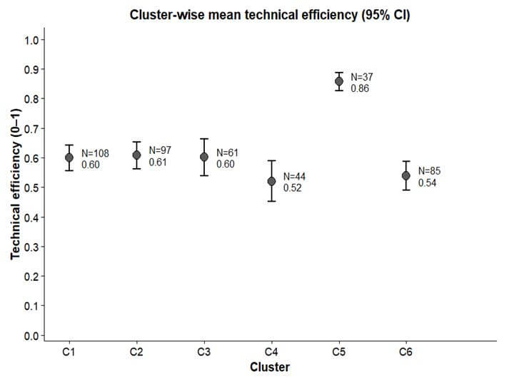
Figure 8. Cluster-specific technical efficiency scores (Model 4).

4.5. Output Effects and Cluster Differences (OLS Estimates)

Table 8 presents OLS estimates of ln(total output) from sequential model specifications. In the initial specification, C5 shows significantly higher output than the reference group (C1), whereas C4 shows significantly lower output. C6 also shows lower output in Models 2 and 3. In the specification including all covariates (M4), only Cluster 5 remains statistically significant (0.496, p < 0.01) after controlling for farm structure, household characteristics, and district effects. The coefficients for the remaining clusters are not statistically significant in this specification. Farm size remains positively and significantly associated with output across models. Relative to marginal holdings, farms operating 1–2 hectares show significantly higher output (0.448, p < 0.01), while holdings above 2 hectares exhibit an even larger effect (0.703, p < 0.01). Improved seed adoption is also positively associated with output (0.315, p < 0.01). Household size is also positively and significantly associated with output. District effects remain substantial: Mandi records higher output than Kangra, whereas Hamirpur records lower output. The results indicate that output differences across clusters are largely explained by structural factors such as farm size and district conditions, with only C5 retaining a significant output advantage in the full specification. This finding is consistent with the efficiency estimates, where C5 also remains statistically distinct in the fully specified model.

Table 8. OLS Estimates for ln (Total Output) with HC1 Robust Standard Errors.

Note: C1 is the reference category. Marginal holding (<1 ha) is the base category. District Kangra is the reference district. Robust standard errors (HC1) are reported in parentheses.

^*** p < 0.01, ^** p < 0.05, ^* p < 0.10.

5. Discussion

The results indicate that maize farmers in the low-hill regions of Himachal Pradesh face different sets of production constraints, rather than a single common set of problems. The six clusters identified include climate variability (C1), wildlife damage (C2), seed access (C3), land fragmentation (C4), mechanization constraint salient (C5), and pest and disease pressure (C6), each representing a distinct production situation. These cluster profiles help explain why farmers experience unequal efficiency and output outcomes in the region. This comparison highlights that whether constraints are within or beyond farmers’ control plays a key role in shaping production performance. As a result, examining technical efficiency and output through cluster-specific constraint profiles provides a clearer understanding of performance differences than analyses based only on average farm characteristics. In this context, results show that maize-growing households in the low-hill zone operate in distinct constraint environments that shape TE and output in consistent ways.

The highest mean technical efficiency (0.86) is observed in C5 (Mechanization-Constraint Salient). This indicates that farms in this cluster benefit from relatively stronger structural conditions, particularly regarding operational scale and input organization. Although mechanization is identified as a salient constraint, the comparatively high efficiency level suggests that production processes are otherwise well aligned with available resources. Evidence from India indicates that labor and machinery shortages continue to limit the adoption of mechanization (Awachat & Sharma, 2024), while improved access to mechanization services enhances timeliness and reduces labor dependence, contributing to higher technical efficiency (Zhu et al., 2025). These findings suggest that the salience of mechanization in this cluster arises at higher levels of operational intensity rather than from basic resource scarcity.

In contrast to the higher efficiency observed in C5, Cluster C2 (Wildlife Damage) exhibits a lower mean technical efficiency (0.61). This efficiency gap is closely associated with wildlife-related disruptions, which raise labor costs through field guarding and lead to production losses. At the farm level, field evidence from Himachal Pradesh indicates that wild boar and monkeys are the dominant crop-raiding species, with farmers reporting frequent incursions and substantial reductions in harvested produce and household income (Mehta et al., 2018). In low-hill regions, nearly 46% of the maize area is exposed to wildlife damage, resulting in a 16–24% decline in cereal productivity and increased production costs due to fencing and watch-and-ward requirements (R. K. Thakur et al., 2022). Government conflict-mapping exercises and regional Himalayan evidence similarly identify wild boar and monkeys as major threats to maize cultivation, with economic losses increasing as wildlife encounter rates rise (Adhikari et al., 2024; Zoological Survey of India, 2020). Wildlife damage represents a largely exogenous pressure. These recurring production losses help explain why farmers in this cluster struggle to consistently operate near their potential.

C1 (Climate Variability) shows low TE (0.60), a pattern also observed in the Western Himalayan region. KC et al. (2022) document that climate change has increased the irregularity of rainfall, snowfall, and precipitation timing across Himalayan farming systems, disrupting field operations and nutrient uptake in major crops. Recent evidence from the Western Himalaya shows that higher Kharif-season temperatures significantly reduce maize yield (Choudhary & Gupta, 2023). District-level analyses from Himachal Pradesh further demonstrate that increased variability in monsoon rainfall and rising maximum temperatures significantly reduce maize productivity, particularly in Kangra, one of the key maize-producing hill districts (Singh et al., 2024). Such timing disruptions make it more difficult for farmers to achieve potential efficiency, even when input management is adequate.

C3 (Seed Access) shows relatively low technical efficiency (0.60) compared to C5, which appears to be linked to difficulties in securing good-quality seed at the appropriate time. Delayed access to preferred seed varieties affects crop establishment and yield realization, with implications for production performance (Gairhe et al., 2021). Related studies emphasize the importance of timely access to quality seed for improved productivity outcomes (Atreya et al., 2025; Nandi, 2024). These findings suggest that unreliable or delayed access to improved seed may limit farmers’ ability to reach potential output levels

The lowest technical efficiency is observed in C4 (Land Fragmentation), with a mean TE of 0.52, followed by C6 (Pest and Disease Pressure) at 0.54. For C6, biological risks such as pest outbreaks and fall armyworm infestation have been shown to generate significant yield losses in maize systems (Ma et al., 2024; Srinivasan et al., 2022), which is consistent with the comparatively lower efficiency observed in this cluster.

In the case of C4, lower efficiency appears linked to structural land fragmentation. Managing multiple small and scattered plots increases supervision requirements and limits the effective use of machinery. Empirical evidence from India consistently shows that land fragmentation raises cultivation costs and reduces farm efficiency (Deininger et al., 2017; Manjunatha et al., 2013), with similar constraints reported in the Western Himalayas (Shukla et al., 2018). These clusters, therefore, operate further from the production frontier relative to other groups, reflecting constraints related to biological risk in C6 and structural scale limitations in C4. While efficiency captures how effectively inputs are converted into output, realized production outcomes remain influenced by additional structural and environmental factors.

The regression results further support these findings. C5 households also record higher output levels, while C6 and C4 exhibit comparatively lower output levels, consistent with the role of constraint environments in shaping outcomes. The results suggest two broad types of production contexts. One is shaped primarily by biophysical and external risks, such as climate variability, wildlife damage, and pest pressure, where short-run adjustment is limited, and efficiency gaps are more evident. The other is characterized by constraints linked to farm structure and management, including seed access, mechanization, and land fragmentation, where performance outcomes appear more responsive to farm-level decisions and institutional support. This distinction helps clarify why efficiency and output differences vary across constraint environments.

The Plackett–Luce ranking results offer complementary evidence on the constraint environment identified through the cluster analysis. They indicate that low returns and rising input costs are widely ranked as the most severe constraints across clusters, while climate-related risks, pest pressure, and wildlife damage also appear among the leading limitations. The concentration of importance around these factors supports the cluster-based finding that production outcomes are shaped primarily by risk- and cost-related pressures rather than by purely farm-specific limitations.

The inefficiency estimates underscore the importance of structural capacity and technology adoption. Larger landholdings are associated with lower inefficiency, consistent with evidence from India showing that land fragmentation and smaller operational scale increase cultivation costs and reduce farm efficiency (Dagar et al., 2021; Deininger et al., 2017). Improved seed use is likewise linked to lower inefficiency, aligning with findings from maize-based systems in India that emphasize the role of input quality in shaping technical performance (Guha & Mandal, 2021). Household size also shows a negative association with inefficiency, suggesting that family labour availability supports more efficient farm management. In contrast, institutional variables do not exhibit statistically significant effects in the full specification, indicating that efficiency differences in this sample are more closely tied to structural and technological factors than to formal program participation.

District patterns reinforce these mechanisms. Kangra and Hamirpur contain more C2 and C6 households, consistent with known wildlife pressure and pest prevalence in these districts, while Mandi’s more balanced constraint mix corresponds to its moderate TE and output. The mean technical efficiency in this study is about 0.60. These values indicate substantial unused production potential among maize-growing households. Comparable patterns are reported for hill maize systems in Sikkim, where Guha and Mandal (2021) find an average TE of around 0.55 and wide variation across agro-climatic zones, suggesting that low-hill maize cultivation typically exhibits considerable heterogeneity in efficiency.

These patterns indicate that differences in technical efficiency and output depend on the dominant constraint environment that farmers face. In clusters affected mainly by climatic risk, wildlife damage, and pest and disease pressure, improvements in efficiency and output are more likely to come from better risk management and timely advisory support than from greater input use. By contrast, clusters characterized by operational constraints—such as delayed or poor-quality seed access, land fragmentation, and limited mechanization—may benefit more from improvements in input timing, access to machinery, and coordination of farm operations. Overall, the findings suggest that institutional support is most effective when aligned with the specific constraints faced by farmers, rather than applied uniformly across different production contexts.

The findings indicate that TE differences in the low-hill zone arise from distinct combinations of climatic risk, wildlife interference, seed-timing conditions, land structure, mechanization access, and pest pressure. These constraints function as production environments that shape farmers’ ability to convert inputs into outputs, and the alignment among empirical clusters, district patterns, and the existing literature reinforces the credibility of this interpretation.

6. Conclusion

The findings from this study indicate that maize-growing households in the low-hill zone operate in structurally distinct constraint environments, which significantly influence their technical efficiency and production outcomes. These findings point to the importance of constraints beyond household characteristics in shaping agricultural performance.

By combining constraint ranking with efficiency estimation, this study provides additional insight into how different production stresses are associated with productivity differences. Rather than assuming homogeneous production conditions, the analysis highlights how heterogeneity in constraints shapes efficiency and output outcomes. The alignment between empirical clusters and known agronomic, ecological, and institutional challenges enhances the credibility of these patterns and helps clarify where policy attention may be most effective. Together, these findings highlight that differences in technical efficiency and output are closely tied to heterogeneity in production constraints rather than to uniform input use alone. From a policy perspective, the results suggest that interventions are likely to be more effective when tailored to the dominant constraint environment farmers face, rather than applied uniformly across heterogeneous production contexts.

As with any empirical analysis, this study has limitations. The data represent one agricultural season, which limits the ability to capture year-to-year climatic variation or long-term adjustment. Ranked constraints reflect farmers’ perceptions, which may differ from measured biophysical conditions. In addition, the study covers three districts, limiting broader generalization. Future research could examine multi-season data, integrate remote-sensing-based agronomic indicators, explore how constraint clusters evolve over time, and assess how targeted interventions reshape efficiency patterns.

CRediT Author Statement: Sudha Kumari: Conceptualization, Methodology, Data Curation, Formal Analysis, Software, Visualization, Writing–original draft, and Writing–review & editing; Rakesh Singh: Supervision, Methodology, Validation, and Writing–review & editing.

Data Availability Statement: The data supporting this study is available from the corresponding author upon reasonable request.

Funding: This research received no external funding.

Conflicts of Interest: The authors declare no conflicts of interest.

IRB Statement: This study was conducted in accordance with institutional ethical guidelines for research involving human participants.

Informed Consent Statement: Informed consent was obtained from all participants involved in the study.

Acknowledgments: The authors would like to thank the anonymous reviewers and the editor for their valuable comments and suggestions, which helped improve the manuscript. The authors also gratefully acknowledge the farmers who participated in the survey and generously shared their time, experiences, and insights for this research.

Abbreviations

The following abbreviations are used in this manuscript:

 

Appendix A

Table A1. Farmers’ characteristics.

Note: n (%) denotes frequency and percentage, respectively.

Table A2. Sensitivity of the Six-Cluster Solution to Linkage Method.

Note. The adjusted Rand index (ARI) measures agreement between cluster partitions. Values between 0.60 and 0.80 indicate strong agreement, suggesting that the six-cluster solution is robust to alternative linkage criteria.

Table A3. Likelihood Ratio Tests (TL vs CD).

Note: LR = 2[LogL (TL) – LogL (CD)]. H0: Cobb–Douglas is sufficient.

Table A4. Model Selection Criteria.

Note: Lower AIC, BIC, and HQIC indicate better model fit. TL = Translog; CD = Cobb–Douglas; HN = Half-normal; TN = Truncated-normal.

Table A5. Correlation Matrix of Technical Efficiency Scores.

Note: Correlations computed using model-specific TE predictions (N = 432).

Table A6. Distribution of Technical Efficiency by Model.

Note: TE is bounded between 0 and 1.

References

Adhikari, J. N., Bhattarai, B. P., & Thapa, T. B. (2024). Correlates and impacts of human–mammal conflict in the central part of Chitwan
Annapurna Landscape, Nepal. Heliyon, 10(4), e26386.
https://doi.org/10.1016/j.heliyon.2024.e26386

Aigner, D., Lovell, C. A. K., & Schmidt, P. (1977). Formulation and estimation of stochastic frontier production function models. Journal of Econometrics, 6(1), 21–37. https://doi.org/10.1016/0304-4076(77)90052-5

Akaike, H. (1974). A new look at the statistical model identification. IEEE Transactions on Automatic Control, 19(6), 716–723. https://doi.org/10.1109/TAC.1974.1100705

Aryal, J. P., Rahut, D. B., Thapa, G., & Simtowe, F. (2021). Mechanisation of small-scale farms in South Asia: Empirical evidence derived from farm households survey. Technology in Society, 65, 101591. https://doi.org/10.1016/j.techsoc.2021.101591

Atreya, K., Gartaula, H. N., & Kattel, K. (2025). Household seed security: A case of maize and wheat seed systems in the mountains of Nepal. Agricultural Systems, 229, 104419. https://doi.org/10.1016/j.agsy.2025.104419

Awachat, S., & Sharma, D. (2024, November 18–20). A review on impact of agricultural mechanization on farm productivity and factors
facilitating the growth of mechanization. 2024 5th International Conference on Data Intelligence and Cognitive Informatics (ICDICI), Tirunelveli, India. https://doi.org/10.1109/ICDICI62993.2024.10810850

Banerjee, H., Goswami, R., Chakraborty, S., Dutta, S., Majumdar, K., Satyanarayana, T., Jat, M. L., & Zingore, S. (2014). Understanding
biophysical and socio-economic determinants of maize (Zea mays L.) yield variability in eastern India. NJAS: Wageningen Journal of Life Sciences, 70–71(1), 79–93. https://doi.org/10.1016/j.njas.2014.08.001

Baral, S., & Bardhan, D. (2016). Multivariate typology of milk producing households in Uttarakhand hills: Explaining profitability in dairy farming. Indian Journal of Agricultural Economics, 71(2), 160–175.
https://doi.org/10.22004/ag.econ.302202

Battese, G. E. (1992). Frontier production functions and technical efficiency: A survey of empirical applications in agricultural economics.
Agricultural Economics, 7(3–4), 185–208. https://doi.org/10.1111/j.1574-0862.1992.tb00213.x

Battese, G. E., & Coelli, T. J. (1995). A model for technical inefficiency effects in a stochastic frontier production function for panel data.
Empirical Economics, 20, 325–332. https://doi.org/10.1007/BF01205442

Bravo-Ureta, B. E., & Pinheiro, A. E. (1993). Efficiency analysis of developing country agriculture: A review of the frontier function literature. Agricultural and Resource Economics Review, 22(1), 88–101. https://doi.org/10.1017/S1068280500000320

Brentari, E., Dancelli, L., & Manisera, M. (2016). Clustering ranking data in market segmentation: A case study on Italian McDonald’s
customers’ preferences. Journal of Applied Statistics, 43(11), 1959–1976.
https://doi.org/10.1080/02664763.2015.1125864

Burnham, K. P., & Anderson, D. R. (2004). Multimodel inference: Understanding AIC and BIC in model selection. Sociological Methods & Research, 33(2), 261–304. https://doi.org/10.1177/0049124104268644

Charnes, A., Cooper, W. W., & Rhodes, E. (1978). Measuring the efficiency of decision making units. European Journal of Operational
Research, 2(6), 429–444. https://doi.org/10.1016/0377-2217(78)90138-8

Chatterjee, S., Dhole, A., Krishnan, A. A., & Banerjee, K. (2023). Mycotoxin monitoring, regulation and analysis in India: A success story. Foods, 12(4), 705. https://doi.org/10.3390/foods12040705

Choudhary, T. F., & Gupta, M. (2023). Analyzing long-run and short-run impacts of climate change on wheat and maize yield in the Western Himalayan Region of India. Climate Change Economics, 14(2), 23500197.
https://doi.org/10.1142/S2010007823500197

Christensen, L. R., Jorgenson, D. W., & Lau, L. J. (1973). Transcendental logarithmic production frontiers. The Review of Economics and
Statistics, 55(1), 28–45. https://doi.org/10.2307/1927992

Coelli, T. J., Rao, D. S. P., O’Donnell, C. J., & Battese, G. E. (2005). An introduction to efficiency and productivity analysis (2nd ed.). Springer New York. https://doi.org/10.1007/b136381

Dagar, V., Khan, M. K., Alvarado, R., Usman, M., Zakari, A., Rehman, A., Murshed, M., & Tillaguango, B. (2021). Variations in technical
efficiency of farmers with distinct land size across agro-climatic zones: Evidence from India. Journal of Cleaner Production, 315, 128109. https://doi.org/10.1016/j.jclepro.2021.128109

Deininger, K., Monchuk, D., Nagarajan, H. K., & Singh, S. K. (2017). Does land fragmentation increase the cost of cultivation? Evidence from India. The Journal of Development Studies, 53(1), 82–98. https://doi.org/10.1080/00220388.2016.1166210

Department of Economics & Statistics. (2022). State statistical abstract 2021–22. Government of Himachal Pradesh.
https://himachalservices.nic.in/economics/pdf/State%20Statistical%20Abstract%20-%202021-22.pdf

Deutschmann, J. W., Duru, M., Siegal, K., & Tjernström, E. (2025). Relaxing multiple agricultural productivity constraints at scale. Journal of Development Economics, 174, 103409. https://doi.org/10.1016/j.jdeveco.2024.103409

Economics, Statistics, and Evaluation Division. (2023). Agricultural statistics at a glance 2023. Government of India, Ministry of Agriculture and Farmers Welfare. Department of Agriculture and Farmers Welfare.
https://nccd.gov.in/uploads/Agricultural_Statistics_at_a_Glance_2023_64c3ac54bf.pdf

Erenstein, O., Jaleta, M., Sonder, K., Mottaleb, K., & Prasanna, B. M. (2022). Global maize production, consumption and trade: Trends and R&D implications. Food Security, 14, 1295–1319. https://doi.org/10.1007/s12571-022-01288-7

Etumnu, C., & Gray, A. W. (2020). A clustering approach to understanding farmers’ success strategies. Journal of Agricultural and Applied Economics, 52(3), 335–351. https://doi.org/10.1017/aae.2020.4

Fonseca, J. R. S. (2013). Clustering in the field of social sciences: That is your choice. International Journal of Social Research Methodology, 16(5), 403–428. https://doi.org/10.1080/13645579.2012.716973

Gairhe, S., Timsina, K. P., Ghimire, Y. N., Lamichhane, J., Subedi, S., & Shrestha, J. (2021). Production and distribution system of maize seed in Nepal. Heliyon, 7(4), e06775. https://doi.org/10.1016/j.heliyon.2021.e06775

Greene, W. H. (2003). Econometric analysis (5th ed.). Pearson Education.

Guha, P., & Mandal, R. (2021). Technical inefficiency of maize farming and its determinants in different agro-climatic regions of Sikkim, India. Indian Journal of Agricultural Economics, 76(2), 225–244.
https://ageconsearch.umn.edu/record/345164/?v=pdf

Hennig, C. (2007). Cluster-wise assessment of cluster stability. Computational Statistics & Data Analysis, 52(1), 258–271. https://doi.org/10.1016/j.csda.2006.11.025

ICAR–Indian Institute of Maize Research. (2022). Annual report 2022. Indian Council of Agricultural Research.
https://iimr.icar.gov.in

Jat, S. L., Jat, H. S., Rakshit, S., Sharma, P. R., Kumar, B., Kakraliya, M., Gathala, M. K., Bijarniya, D., Kalwania, K. C., Singh, Y., Choudhary, M., & Jat, M. L. (2025). Maize as an alternative to resource-intensive rice: Empirical insights from on-farm participatory study under diverse agricultural scenarios in the Indo-Gangetic Plains of Northwestern India. Frontiers in Sustainable Food Systems, 9, 1700854. https://doi.org/10.3389/fsufs.2025.1700854

Johnson, S. C. (1967). Hierarchical clustering schemes. Psychometrika, 32(3), 241–254.
https://doi.org/10.1007/BF02289588

Jondrow, J., Lovell, C. A. K., Materov, I. S., & Schmidt, P. (1982). On the estimation of technical inefficiency in the stochastic frontier
production function model. Journal of Econometrics, 19(2–3), 233–238.
https://doi.org/10.1016/0304-4076(82)90004-5

Kaufman, L., & Rousseeuw, P. J. (2009). Finding groups in data: An introduction to cluster analysis (2nd ed.). Wiley.

KC, K. B., Tzadok, E., & Pant, L. (2022). Himalayan ecosystem services and climate change driven agricultural frontiers: A scoping review. Discover Sustainability, 3, 35. https://doi.org/10.1007/s43621-022-00103-9

Kharwal, D., Sharma, P. K., & Kumar, A. (2025). Yield losses caused by lepidopteran pest complex infesting maize in Himachal Pradesh, India. Asian Research Journal of Agriculture, 18(4),158–165. https://doi.org/10.9734/arja/2025/v18i4775

Kumar, P., Sarda, R., Yadav, A., Ashwani, Gonencgil, B., & Rai, A. (2025). Farmer’s perception of climate change and factors determining the adaptation strategies to ensure sustainable agriculture in the cold desert region of Himachal Himalayas, India. Sustainability, 17(6), 2548. https://doi.org/10.3390/su17062548

Kumari, S., & Sharma, H. R. (2018). Farmers’ perception on environmental effects of pesticide use, climate change and strategies used in
mountain of Western Himalaya. International Journal of Agricultural Science and Research, 8(1), 57–68.
https://ssrn.com/abstract=3172041

Kumar, S., & Singh, A. K. (2023). Modeling the effects of climate change on agricultural productivity: Evidence from Himachal Pradesh, India. Asia-Pacific Journal of Regional Science, 7, 521–548. https://doi.org/10.1007/s41685-023-00291-w

Kumbhakar, S. C., Parmeter, C. F., & Zelenyuk, V. (2021). Stochastic frontier analysis: Foundations and advances. In S. C. Ray, R. G.
Chambers, & S. C. Kumbhakar (Eds.), Handbook of production economics (pp. 1–40). Springer Singapore. https://doi.org/10.1007/978-981-10-3450-3_9-2

Manjunatha, A. V., Anik, A. R., Speelman, S., & Nuppenau, E. A. (2013). Impact of land fragmentation, farm size, land ownership and crop diversity on profit and efficiency of irrigated farms in India. Land Use Policy, 31, 397–405. https://doi.org/10.1016/j.landusepol.2012.08.005

Ma, Z., Wang, W., Chen, X., Gehman, K., Yang, H., & Yang, Y. (2024). Prediction of the global occurrence of maize diseases and estimation of yield loss under climate change. Pest Management Science, 80(11), 5759–5770.
https://doi.org/10.1002/ps.8309

Meeusen, W., & van Den Broeck, J. (1977). Efficiency estimation from Cobb-Douglas production functions with composed error. International Economic Review, 18(2), 435–444. https://doi.org/10.2307/2525757

Mehta, P., Negi, A., Chaudhary, R., Janjhua, Y., & Thakur, P. (2018). A study on managing crop damage by wild animals in Himachal Pradesh. International Journal of Agriculture Sciences, 10(12), 6438–6442.
https://bioinfopublication.org/pages/article.php?

Nandi, S. (2024). Impact of formal seed sources on smallholder farming in India: Evidence from NSS survey using propensity score matching. Indian Journal of Agricultural Economics, 79(3), 709–724. https://doi.org/10.63040/25827510.2024.03.026

Negi, G. C. S., Samal, P. K., Kuniyal, J. C., Kothyari, B. P., Sharma, R. K., & Dhyani, P. P. (2012). Impact of climate change on the western Himalayan mountain ecosystems: An overview. Tropical Ecology, 53(3), 345–356.

Organisation for Economic Co-operation and Development, & Food and Agriculture Organization of the United Nations. (2025). OECD-FAO Agricultural outlook 2025–2034. https://doi.org/10.1787/601276cd-en

Rajkhowa, P., & Kubik, Z. (2021). Revisiting the relationship between farm mechanization and labour requirement in India. Indian Economic Review, 56, 487–513. https://doi.org/10.1007/s41775-021-00120-x

Ranum, P., Peña-Rosas, J. P., & Garcia-Casal, M. N. (2014). Global maize production, utilization, and consumption. Annals of the New York Academy of Sciences, 1312(1), 105–112. https://doi.org/10.1111/nyas.12396

Rasool, A., & Abler, D. (2023). Heterogeneity in US farms: A new clustering by production potentials. Agriculture, 13(2), 258. https://doi.org/10.3390/agriculture13020258

R Core Team. (2025). R: A language and environment for statistical computing (Version 4.5.1). R Foundation for Statistical Computing. https://www.r-project.org/

Roy, P., Hansra, B. S., Burman, R. R., Bhattacharyya, S., Roy, T. N., & Ahmed, R. (2022). Can farm mechanization enhance small farmers’ income? Lessons from Lower Shivalik Hills of the Indian Himalayan Region. Current Science, 123(5), 667–676. https://doi.org/10.18520/cs/v123/i5/667-676

Salama, I. A., & Quade, D. (1982). A nonparametric comparison of two multiple regressions by means of a weighted measure of correlation. Communications in Statistics - Theory and Methods, 11(11), 1185–1195.
https://doi.org/10.1080/03610928208828304

Schwarz, G. (1978). Estimating the dimension of a model. The Annals of Statistics, 6(2), 461–464.
https://doi.org/10.1214/aos/1176344136

Shukla, R., Chakraborty, A., Sachdeva, K., & Joshi, P. K. (2018). Agriculture in the Western Himalayas – An asset turning into a liability.
Development in Practice, 28(2), 318–324. https://doi.org/10.1080/09614524.2018.1420140

Singh, P., Guleria, A., Guleria, C., & Vaidya, M. K. (2024). The Climatic variability and its impact on maize and wheat yield in Himachal
Pradesh. MAUSAM, 75(3), 669–678. https://doi.org/10.54302/mausam.v75i3.5882

Srinivasan, T., Shanmugam, P. S., Baskaran, V., Kavitha, Z., Yasodha, P., Ravi, M., Sathiah, N., Rabindra, R. J., Krishnamoorthy, S. V., Vinothkumar, B., Suganthy, A., Balakrishnan, N., Backiyaraj, S., Arulkumar, G., Jeyarani, S., Shanthi, M. Srinivasan, M. R., Justin, G. L., & Prabakar, K. (2022). Estimation of avoidable yield loss in maize (Zea mays L.) caused by the fall armyworm Spodoptera
frugiperda (J.E. Smith) (Noctuidae: Lepidoptera). Ecology, Environment & Conservation, 28(4), 1946–1957.
https://doi.org/10.53550/EEC.2022.v28i04.044

Srivastava, R. K., Panda, R. K., & Chakraborty, A. (2021). Assessment of climate change impact on maize yield and yield attributes under
different climate change scenarios in eastern India. Ecological Indicators, 120, 106881.
https://doi.org/10.1016/j.ecolind.2020.106881

Stevenson, R. E. (1980). Likelihood functions for generalized stochastic frontier estimation. Journal of Econometrics, 13(1), 57–66. https://doi.org/10.1016/0304-4076(80)90042-1

Thakur, A. N. (2024). Input use and socio-economic status of farmers: A case of paddy cultivation in India. Indian Journal of Agricultural
Economics, 79(3), 686–694. https://doi.org/10.63040/25827510.2024.03.024

Thakur, R. K., Walia, A., Mehta, K., Kumar, V., & Lal, H. (2022). Economic assessment of crop damages by animal menace in mid hill regions of Himachal Pradesh. The Indian Journal of Animal Sciences, 92(4), 484–491.
 https://doi.org/10.56093/ijans.v92i4.124173

Turner, H. L., van Etten, J., Firth, D., & Kosmidis, I. (2020). Modelling rankings in R: The PlackettLuce package. Computational Statistics, 35, 1027–1057. https://doi.org/10.1007/s00180-020-00959-3

United States Department of Agriculture Foreign Agricultural Service. (2025). Biofuels annual: India. United States Department of Agriculture.
https://apps.fas.usda.gov/newgainapi/api/Report/DownloadReportByFileName?fileName=Biofuels%20Annual_New%20Delhi_India_IN2025-0031.pdf

Wang, H., Ren, H., Han, K., Zhang, L., Zhao, Y., Liu, Y., He, Q., Li, G., Zhang, J., Zhao, B., Ren, B., & Liu, P. (2023). Experimental
assessment of the yield gap associated with maize production in the North China Plain. Field Crops Research, 295, 108897. https://doi.org/10.1016/j.fcr.2023.108897

Zhu, Y., Wang, G., Du, H., Liu, J., & Yang, Q. (2025). The effect of agricultural mechanization services on the technical efficiency of cotton production. Agriculture, 15(11), 1233. https://doi.org/10.3390/agriculture15111233

Zoological Survey of India. (2020). Inception report on human–wildlife conflict management baseline survey and development of comprehensive strategy for its mitigation in selected districts of Himachal Pradesh. Ministry of Environment, Forests and Climate Change.