Research on the Impact of Homestead Withdrawal on Rural Residents’ Well-Being—An Analysis of the Mediating Effect of Non-Agricultural Employment

1. Introduction

The rapid pace of industrialization and urbanization in China is transforming the nation from predominantly rural to a society characterized by a dynamic urban-rural interplay. The weakening connections between farmers and land, coupled with their evolving relationships with rural communities, are reshaping rural employment patterns and lifestyles (Chen et al., 2022). However, when homesteads are relinquished, households—the primary beneficiaries—often receive a smaller portion of the appreciation than anticipated (He et al., 2020). Compensation formulas typically overlook the higher cost of living at resettlement sites and the weak incentives for off-farm employment (Gao & Li, 2020); thus, households receive less compensation than expected, which undermines their living standards. Homestead withdrawal is a cornerstone of rural land-system reform; it addresses inefficient land use and provides a crucial avenue for improved resource allocation (Zou et al., 2020). However, it can stimulate off-farm employment, enhance household well-being, and foster balanced, healthy rural development. From 2017 to 2025, the annual “No. 1 Central Document” repeatedly singled out rural homestead reform, pilot areas actively promoted voluntary, compensated withdrawal.

President Xi Jinping has emphasized farmers’ well-being, calling for “beautiful, ecologically livable villages that enhance our rural people’s sense of gain and happiness.” The first round of national pilot programs has concluded, with regions formulating policies tailored to their specific needs. However, the literature—both domestic and international—still concentrates on willingness to exit (Han & Liu, 2021; Niu et al., 2022), exit behavior (Hu et al., 2020; Sun & Chen, 2021), and exit mechanisms (Chen et al., 2016; Zhang & Bao, 2019). However, systematic studies on the impact of homestead withdrawal on rural residents’ well-being remain scarce. The “Deepening Rural Homestead Reform Pilot Program” (June 2020) and the subsequent nationwide launch of a second pilot wave (September 2020) established an institutional framework that facilitated the unlocking of idle homesteads, expanded property income channels, and enhanced rural welfare. This was achieved by exploring voluntary and paid exit mechanisms, ensuring collective ownership, and safeguarding farmers’ rights to homesteads and property. Through the monetization of rural land, this policy can increase households’ property income and enable them to share in the benefits of reform (Qu et al., 2012), thereby enhancing their quality of life. However, some scholars caution that unreasonable compensation and resettlement arrangements may undermine farmers’ property rights (Han et al., 2018; Jia et al., 2009). Empirically, one fuzzy-evaluation study found that exit enhances economic well-being (Yang et al., 2018), whereas Yi et al. (2010) reported a deterioration. Improving residents’ well-being can dismantle barriers in social resource allocation, enhance life satisfaction across different strata, eliminate urban-rural, regional, and sectoral disparities, resolve historical grievances, and prevent new imbalances (Wang, 2021). This is not only a prerequisite for equitable wealth distribution but also an effective route to high-quality development and common prosperity (Ding, 2021). Moreover, well-being lies at the heart of ecological civilization and sustainable development research (Huang et al., 2016).

Guided by Sen’s capability approach, this study utilizes field data collected from the western counties of Dezhou, Shandong, encompassing villages in various locations. Through the integration of theoretical and empirical analyses, this study assesses how homestead withdrawal impacts multiple dimensions of rural residents’ well-being, furnishes evidence for refining exit mechanisms and deepening reform, and proposes policy recommendations that more effectively safeguard farmers’ homestead rights, enhance land-use efficiency, and alleviate local shortages of construction land.

2. Theoretical Analysis and Research Hypotheses

The mechanism by which homestead withdrawal impacts rural residents’ well-being can be elucidated through two interrelated channels. First, by reshaping the physical environment where households farm and reside, the policy modifies production routines and daily life. The magnitude of households’ livelihood capital—natural, physical, financial, human, and social—determines whether the new configuration increases or decreases total income. Second, after homesteads are relinquished, local governments typically also supply (i) vocational training aimed at off-farm jobs and (ii) upgraded transportation, telecommunications, and other public infrastructure. These interventions lead to a reallocation of household production factors, create new off-farm earning opportunities, and thus alter the total family income. Furthermore, the program enhances farmers’ access to information regarding wage employment, increases their expected off-farm wages, and expedites labor transfer to non-agricultural sectors, all of which contribute tock into higher subjective and objective well-being.

2.1. Theoretical Framework

We establish a three-node framework that connects homestead withdrawal, off-farm employment, and rural residents’ well-being. The model posits that the impact of households’ decision to withdraw from the homestead on their well-being is mediated by the degree of rural labor transfer to off-farm activities. A graphical representation of the framework is shown below (Figure 1).

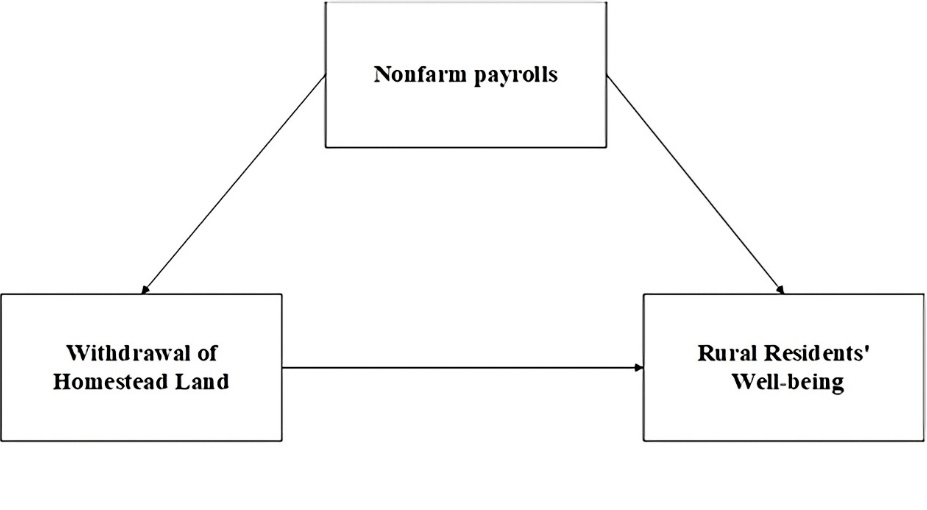
Figure 1. Theoretical Model Diagram.

2.2. Direct Effect of Household Homestead Withdrawal on Rural Residents’ Well-Being

The “rational-peasant” hypothesis posits that, in order to maximize expected utility, households assess the marginal benefits and costs prior to surrendering their homesteads. Empirically, land-transfer decisions are motivated by the objective of maximizing household income, and multiple studies have demonstrated that homestead withdrawal exerts a positive net impact on total family revenue (Sun & Zhao, 2020). Research on impoverished rural households indicates that leasing out farmland serves as a significant catalyst for wealth accumulation; specifically, the withdrawal of rural residential land affects the stock of residents’ financial capital and physical capital through means such as asset monetization and equity replacement. Non-agricultural employment optimizes the quality of human capital and financial capital through skill acquisition and income growth. Changes in these dimensions of livelihood capital will further affect different well-being dimensions such as economic income, health security, social integration, and psychological satisfaction. The flow of farmland (either out of or into the household) reshapes the labor allocation among family members and increases aggregate income (Zhou et al., 2020). Therefore, reforming the homestead system is imperative. Deepening the reform can unlock the latent property value of homesteads, activate idle land resources, and narrow the development gaps among regions, villages, and individuals, thereby fostering common prosperity among rural residents (Cao & Geng, 2022) and enhancing their well-being.

The multidimensional and dynamic impact of homestead withdrawal on rural well-being necessitates a comprehensive analysis, which can be enriched by empirical studies and theoretical frameworks such as the Sustainable Livelihoods Framework, Sen’s Capability Approach, and social exclusion theory. The homestead, as the core natural and physical capital of rural households, plays a pivotal role in shaping their livelihood strategies. Once surrendered through monetary compensation or spatial relocation, it directly influences their transition into off-farm employment and the reallocation of assets. In the short run, the Change may enhance economic well-being by increasing disposable income and improving living standards. However, insufficient compensation, investment risks, or the breakdown of social networks may subject households to long-term poverty or social exclusion. Furthermore, the impacts are not limited to the economic realm; they extend to social, psychological, and environmental aspects. Therefore, a dynamic evaluation mechanism combined with a differentiated policy design is needed to balance efficiency and equity and achieve sustainable livelihoods and simultaneous improvements in multidimensional well-being. Specifically, the withdrawal of rural residential land affects the stock of residents’ financial capital and physical capital through means such as asset monetization and equity replacement. Non-agricultural employment optimizes the quality of human capital and financial capital through skill acquisition and income growth. Changes in these dimensions of livelihood capital will further affect different well-being dimensions such as economic income, health security, social integration, and psychological satisfaction.

Based on the above discussion, we propose the following:

Hypothesis 1: Homestead withdrawal significantly and positively affects rural residents’ well-being.

2.3. The Mediating Role of Off-Farm Employment

Since the start of reform and opening-up, China’s economic structure has undergone a profound transformation from a centrally planned to a market-oriented system, with the state playing a pivotal guiding role. The development of secondary and tertiary industries has shifted economic growth away from agriculture, driving the coordinated evolution of all three sectors. Continuous industrial upgrading and increased urban non-agricultural job supply have facilitated rural labor migration to cities and accelerated rural household differentiation (Sun et al., 2019). The homestead withdrawal policy has intensified this process: it raises agricultural marginal costs while reducing labor migration transaction costs, making off-farm work a preferred choice for many households. After withdrawing homesteads, families often purchase urban apartments or move to government-provided resettlement housing, increasing spatial and temporal distances to their remaining farmland (Mao et al., 2017), which drives a self-reinforcing shift to areas with better transportation and more jobs, turning off-farm employment into a prevalent trend. Existing studies have explored how household differentiation shapes employment decisions, but rarely treat homestead withdrawal as an independent, multi-channel policy intervention. This theoretical-practical gap is reflected in household decision discrepancies, family background’s influence on career choices, and misalignment between education and job market demands. From an occupational differentiation perspective, the one-time homestead withdrawal subsidy is generally insufficient to cover new rural housing or urban home purchase costs (Yan et al., 2017), forcing households to seek off-farm income. Meanwhile, expanded social networks and younger generations’ evolving career aspirations strengthen the desire to leave agriculture and withdraw homesteads, further promoting off-farm transition.

Motivationally, off-farm employment is driven by the prospect of higher and more diversified earnings—anticipated wages in industry and services significantly exceed agricultural labor opportunity costs (Wang & Cai, 2025). Some workers even plan to settle permanently in towns and cities, engaging in secondary and tertiary sector jobs. In summary, the intricate interaction between homestead withdrawal and off-farm employment remains under-theorized. Research on issues such as non-farm employment’s impact on homestead withdrawal and its poverty reduction mechanisms is essential to disentangle these factors, understand how policies reshape household differentiation, and ultimately affect rural well-being.

Based on the preceding analysis, the following research hypothesis is formulated.

Hypothesis 2: Off-farm employment plays a mediating role in the impact of homestead withdrawal on rural residents’ well-being.

3. Data Sources and Research Methods

3.1. Data Source

The data used in this study were obtained from a random sampling survey conducted in counties in western Shandong Province from March to June 2025, involving random interviews with some township cadres and rural households. To ensure the representativeness of the research subjects, a multi-stage random sampling method was adopted. The focus of this study is to understand farmers’ specific perceptions of the rural residential land withdrawal issue and their willingness to participate in the actual withdrawal process.

Shandong’s regional development strategy has long privileged the eastern prefectures, resulting in the gradual impoverishment of western counties and exacerbating the east-west disparity. Since 2020, the provincial government has designated western Shandong as a top priority for balanced growth. To substantiate this new policy orientation, we selected three western counties where homestead withdrawal pilot programs have been implemented. A stratified sampling approach was employed in conjunction with face-to-face interviews to exhibit high reliability and completeness. The questionnaire encompassed household demographics, homestead-exit status, and village-level characteristics. The final sample consists of 410 farm households selected from nine administrative villages across six townships, spanning one city (Yucheng) and two counties (Wucheng and Xiajin). Among these households, 178 had already surrendered their homesteads, 227 had not, and five questionnaires were discarded, resulting in an effective response rate of 99%.

3.2. Variable Selection and Definition

3.2.1. Dependent Variable: Rural Residents’ Well-Being

Based on the Sustainable Livelihoods Framework and previous studies by Luo et al. (2022), Li et al. (2022), and Peng et al. (2024), we construct a multidimensional well-being index grounded in Amartya Sen’s capability approach. As shown in the data in Table 1, four dimensions were retained: (i) economic conditions, as measured by GDP and GNI, (ii) life satisfaction, encompassing cognitive and emotional aspects, (iii) health status, with a focus on the impact of economic factors, and (iv) social networks, reflecting interpersonal and societal harmony. The evaluation of each dimension was conducted through the application of a comprehensive set of distinct indicators, as demonstrated in the construction of well-being indices detailed in the references. An entropy-weighting procedure that combines objective dispersion with subjective expert scoring was used to derive indicator-specific weights, yielding a continuous composite index. The weights were then applied to the survey data to generate a cardinal well-being score for each respondent, ensuring that changes in rural residents’ well-being were measured with maximum precision, as demonstrated in studies that have constructed happiness indices for urban and rural populations.

Table 1. Construction of the Rural Residents’ Well-Being Indicator System.

3.2.2. Core Explanatory Variable

The withdrawal of homestead land is chosen as the core explanatory variable, which indicates whether households have withdrawn their homestead land, with the categories defined as “Yes = 1, No = 0.” A value of 1 denotes that the household has withdrawn its homestead land, whereas a value of 0 indicates that the household has not done so. Among the 505 valid sample questionnaires collected, 178 correspond to households that have withdrawn homestead land, and 227 correspond to households that have not.

3.2.3. Mediating Variable

Non-agricultural employment was selected as the mediating variable. Following the methodology of Zhou and Yang (2025) and Qiu and Luo (2017), the degree of non-agricultural employment was measured by the proportion of non-agricultural labor force to the total labor force, treated as a continuous variable.

3.2.4. Control Variables

Control variables encompass household head characteristics (e.g., age, educational attainment, and health status), household attributes, homestead characteristics, and production/operational features. Household head characteristics, which include age, educational attainment, and health status, are crucial as they influence various aspects of family life, such as health data tracking, educational and medical expenditures, and overall household consumption patterns. Specific secondary variables are illustrated in Table 2.

Table 2. Variable Selection and Selection Basis.

3.3. Model Specifications

Since homestead withdrawal is a self-selected behavior, the observed differences in welfare indicators may arise not from the withdrawal act itself but from the pre-existing heterogeneity in household-head and family characteristics. To mitigate self-selection bias, we employ Propensity Score Matching (PSM), which pairs households that surrendered their homesteads (treated group) with those that did not (control group), ensuring that both groups are observably similar.

The procedure unfolds in two stages. First, we specify and estimate a homestead-withdrawal decision equation; all computations are carried out with Stata 17.0 to ensure high-quality matching (Sun & Zhao, 2020; Si et al., 2018), as demonstrated by the application of advanced statistical techniques such as Propensity Score Matching (PSM) and Coarsened Exact Matching (CEM) in the references. Second, by maintaining constant external conditions and utilizing a matched sample, we apply Propensity Score Matching (PSM) to ascertain the causal impact of withdrawal on the well-being of rural residents. The detailed steps are as follows:

(1)  Use a Logit model to predict each household’s conditional probability of exiting the homestead:

 (1)

Here,means that farmers have withdrawn from homesteads;means that the farmers have not withdrawn from the homestead;represents observable farmer characteristics (covariates).

(2)  The treatment and control groups will be matched. In order to verify the robustness of the matching results, four matching methods were selected: minimum nearest neighbor matching, caliper matching, kernel matching, and local linear matching.

(3)  Calculate the average treatment effect (ATT). Based on the matching sample, the difference in the well-being status of withdrawn and non-withdrawn farmers is compared, and the impact coefficient of homestead withdrawal on farmers is obtained, that is, the average treatment effect in the model (ATT):

 (2)

represents the welfare status of the first farmer participating in the withdrawal of homestead,means that the welfare status of the first farmer does not participate in the withdrawal of homestead land. Under the assumption, is the average treatment effect of homestead withdrawal on the well-being of farmers.

(4)  The matching test of the PSM model, i.e., the common branch domain test and the balance test (Liang et al., 2017). Table 2 lists the descriptive statistical analysis of the main variables in this study.

4. Empirical Testing and Results Analysis

4.1. The Impact of Homestead Withdrawal on Multidimensional Poverty Reduction: An Empirical Analysis

4.1.1. Analysis of Basic Characteristics of Farmhouse Households

All data in this chapter are derived from the research team’s field investigations. In the study of counties in western Shandong Province, it was found that 178 households in the sample relinquished their homestead land use rights, influenced by objective economic factors and a herd mentality stemming from observing the number of other households that had already withdrawn. Conversely, 227 households did not relinquish their rights, likely due to differing economic considerations or a lack of motivation to withdraw. See Table 2 and Table 3 for details.

Table 3. Analysis of Basic Characteristics of Farmhouse Households.

Combining Table 3 and the descriptive statistics in Table 2, the following patterns emerge. Regarding the outcome variable, the means of the four rural-well-being dimensions show a difference of no more than 0.2, indicating villagers’ relatively consistent priorities. As for the key explanatory variable, most households indicate a willingness to surrender their homestead. Concerning the mediator, more than two-thirds of families have at least one member involved in off-farm labor, whereas only a small minority have relatives or friends employed in the public sector or non-farm enterprises. Control variables can be categorized into four domains: head-of-household traits, household characteristics, homestead attributes, and production-management features.

(1)  Head-of-household characteristics

Age is evenly distributed, with a mean age of 42; 32.84% are aged 50 or older. Junior-middle-school graduates make up 64.69% of the sample, while only 6.91% have completed senior high school or above, reflecting the typical educational profile of western Shandong.

(2)  Household characteristics

Labor-force participants constitute 72.84% of household members, and the proportion working off-farm continues to increase. The number of dependants, presence of a village cadre, and the frequency of kin visits are all stable.

(3)  Homestead characteristics

Thanks to recent land titling campaigns, 66.1% of the plots have been formally certified. The distance to the nearest town varies uniformly across the sample, highlighting the representativeness of the study area.

(4)  Production and management characteristics

Recent data indicate that the rural per-capita disposable income has reached 23,119 yuan in 2024, marking a substantial increase from previous years and reflecting the ongoing improvement in rural income realities.

As shown in Table 4, after homestead withdrawal, both economic conditions and life satisfaction exhibit significant mean changes, with improvements observed and statistical significance at the 1% level. However, changes in interpersonal relationships are not statistically significant. Regarding household head characteristics, the mean educational attainment increased by 0.227, which is statistically significant at the 1% level. The household head’s age and health status showed changes, but were not statistically significant. In terms of family characteristics, the mean number of frequently visiting relatives and friends increased by 0.189, with statistical significance at the 5% level, while changes in household size and number of dependents were insignificant. Regarding homestead characteristics, the mean homestead area decreased significantly at the 1% level; the mean homestead title status showed a slight increase at the 10% level; and the mean distance to the central town decreased but was not statistically significant. Additionally, the mean non-agricultural employment rate increased significantly by 0.043 at the 1% level.

Table 4. Statistical Description of Indicator Mean Differences: Homestead-Withdrawing vs. Non-Withdrawing Households.

Note: ***, **, and * indicate significance at the 1%, 5%, and 10% levels, respectively.

4.1.2. Propensity Score Matching

Following the counterfactual analysis steps of PSM, we selected and evaluated covariates that affect the health of core household members to match samples between the experimental and control groups. The estimation results derived from the Logit model are presented in Table 5.

Table 5. Propensity Score Matched Logit Regression Results

Indicator type	Variable name	Coefficient	Standard error	t-value	Significance
Characteristics of the head of the household	age	−0.013	0.006	−2.017	0.044*
	Educational level	0.374	0.099	3.897	0.000**
	Health level	0.636	0.198	3.136	0.002**
Family characteristics	Family population	0.019	0.074	0.276	0.619
	The number of people to be supported and supported by the family	0.035	0.120	0.569	0.570
	Are there any party members at home?	0.447	0.217	2.075	0.038*
	Are there any village cadres at home?	0.382	0.225	1.62	0.106
	Family livelihood methods	0.074	0.087	0.839	0.402
	The number of relatives and friends who often walk around the house	0.110	0.089	1.138	0.256
Homestead characteristics	Whether the homestead is confirmed	0.621	0.264	2.664	0.008**
	Homestead area	0.138	0.088	1.278	0.202
	Homestead type	−0.372	0.144	−2.918	0.004**
Production and operation characteristics	Is there any outflow of farmland at home	0.803	0.242	3.84	0.000**
	The area of cultivated land operated by the family	−0.705	0.096	−8.685	0.000**
	Household agricultural income	0.051	0.017	3.0112	0.003*
Statistical tests		Pseudo R²		0.343
		LR chi2(15)		294.99
		Prob﹥chi2		P = 0.00

Studies employing Logistic regression models, such as those detailed in the references, have consistently shown that educational attainment and self-reported health status are significant predictors of farmers’ willingness to withdraw from homesteads. For instance, the research detailed in Table 4 of the original document indicates that these factors positively and significantly influence the likelihood of homestead withdrawal, with higher levels of education and better self-reported health status correlating with a greater probability of exit. Shifting focus to household characteristics, the presence of a Communist Party member in the household is positively correlated with the decision to withdraw at the 5% significance level, In contrast, the number of dependents (children and elderly), the number of influential acquaintances, and whether any household member serves as a village cadre do not reach the conventional significance thresholds, and thus cannot reliably distinguish between participants and non-participants. Regarding homestead attributes, formal titling significantly increases the propensity to exit (p < 0.01), whereas non-residential homestead types significantly reduce this propensity (p < 0.01). A study on the impact of livelihood resilience on farmers’ willingness to exit land contracts reveals that leasing out farmland and a higher share of household income from agriculture positively influence the probability of withdrawal, while larger areas of contracted farmland under household cultivation have a negative impact, all at the 1% significance level.

4.2. Measuring the Impact of Homestead Withdrawal on Rural Residents’ Well-Being

4.2.1. Propensity Score Matching

To assess the net impact of homestead withdrawal on rural residents’ well-being, we utilize four distinct matching estimators: nearest-neighbour matching, radius (caliper) matching, kernel matching, and local-linear-regression matching. Table 6 presents the findings. Under the nearest-neighbor specification, 203 treated households are successfully matched, whereas 24 are excluded due to the common-support restriction; 162 control households are matched, with 16 being discarded, resulting in a matched sample. A sample of 365 observations was used, with 40 observations dropped in total. The post-matching balance is satisfactory. The average treatment effect on the treated (ATT) is 0.051 and is highly significant at the 1 % level, indicating that participation in homestead withdrawal indeed raises the rural well-being index. Although the magnitude is smaller than the raw pre-matching difference, the estimate exhibits greater credibility. To verify robustness, we re-estimate the ATT using radius matching and kernel matching methods. Although point estimates differ slightly across various specifications, all four methods exhibit quantitatively similar outcomes, which underscores the robustness of the findings.

Table 6. Balance test results before and after propensity score matching.

Variable	Matching method	Matching Number	Processing group	Control group	Total sample	Average Treatment Effect (ATT)	Standard error	T Statistics
countryside inhabitant welfare	Minimum Nearest Neighbor Matching	supported	203	162	365	0.051	0.020	2.59
		Not supported	24	116	40
	Radius matching	supported	214	163	377	0.049	0.027	1.86
		Not supported	13	15	28
	Nuclear matching	supported	214	163	377	0.047	0.021	2.26
		Not supported	13	15	28
	Local linear Regression matching	supported	214	163	377	0.046	0.027	1.74
		Not supported	13	15	28

4.2.2. Hypothesis Testing: Balance Analysis

This section evaluates the balancing property to test the credibility and robustness of the propensity-score matching results. The fundamental requirement for propensity score matching is that, post-matching, the means of all covariates should not significantly differ between the treatment and control groups, ensuring covariate balance. The degree of balance between groups in randomized controlled trials is often assessed using Standardized Mean Differences (SMDs), which allow for the comparison of mean differences across studies that use different measurement scales. The closer the post-match SMD is to zero, the better the balance; An SMD below 10% is generally considered to indicate a satisfactory level of balance between groups, as suggested by Cohen’s guidelines, where SMD values less than 0.1 typically represent good balance. The table reports the balance diagnostics for every control variable.

Table 7 demonstrates that, among head-of-household characteristics, the standardized bias of all three variables decreases significantly after matching and approaches zero, indicating a satisfactory balance. Within household-level attributes, only the absolute standardized bias of the head’s schooling slightly surpasses 10 percent; all other variables remain comfortably below this threshold. For homestead characteristics, every covariate bias is reduced to nearly zero, whereas in production-management traits only the indicator “whether farmland has been leased out” slightly exceeds 10 percent, while the rest are well below this level. Overall, the treated and control households exhibit balanced distributions across all four dimensions.

Table 7. Propensity Score Matching.

Control variables	Sate	Normalization deviation (%)	Reduction in standardized deviation (%)	t-value	p-value
age	Before matching	3.9%	79.0%	0.39	0.017
	After matching	−0.8%		−0.07	0.942
education	Before matching	23.1%	45.5%	2.32	0.001
	After matching	12.6%		1.16	0.245
health	Before matching	34.8%	60.6%	3.40	0.001
	After matching	−13.7%		−1.40	0.163
Population	Before matching	−7.2%	21.4%	−0.72	0.000
	After matching	5.7%		0.52	0.108
Maintenance	Before matching	19.0%	77.1%	1.89	0.361
	After matching	4.3%		0.41	0.617
Party	Before matching	23.2%	42.7%	2.32	0.089
	After matching	9.3%		1.19	0.808
Cadre	Before matching	98.3%	97.7%	9.70	0.000
	After matching	−2.3%		−0.23	0.564
Make a living	Before matching	2.2%	34.7%	0.22	0.192
	After matching	1.5%		−0.13	0.461
Relatives	Before matching	15.5%	90.4%	1.54	0.168
	After matching	−1.5%		−0.13	0.468
Confirmation	Before matching	6.5%	70.1%	0.65	0.211
	After matching	1.9%		0.18	0.622
Area	Before matching	19.5%	47.9%	1.95	0.000
	After matching	−10.2%		−0.96	0.561
Type	Before matching	−20.3%	86.4%	−2.04	0.000
	After matching	−2.8%		−0.25	0.749
Farmland	Before matching	65.6%	83.5%	6.63	0.000
	After matching	10.8%		0.90	0.042
Arable land	Before matching	−128.6%	93.7%	−12.90	0.000
	After matching	−8.1%		−0.75	0.665
Revenue	Before matching	−32.6%	95.3%	−3.27	0.001
	After matching	−1.5%		1.02	0.307

To visualize these results, we employ Stata 17.0 to plot the changes in standardized bias for each control variable (see Figure 2). After applying propensity-score matching, biases are markedly reduced and cluster around zero, which aligns with the balancing hypothesis and confirms the effectiveness of the matching procedure.

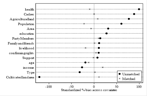
Figure 2. Variable Standardization Deviation Reduction Degree Chart.

4.2.3. Common Support Domain Test

The common-support test serves as an additional prerequisite for ensuring the validity of propensity-score matching. By comparing the kernel-density curves, along with the overlapping support regions, of the treatment and control samples before and after matching, we can assess whether the matching procedure has generated a high-quality counterfactual. Figure 3 and Figure 4 present the kernel-density plots for the homestead-withdrawal group and the non-withdrawal group:

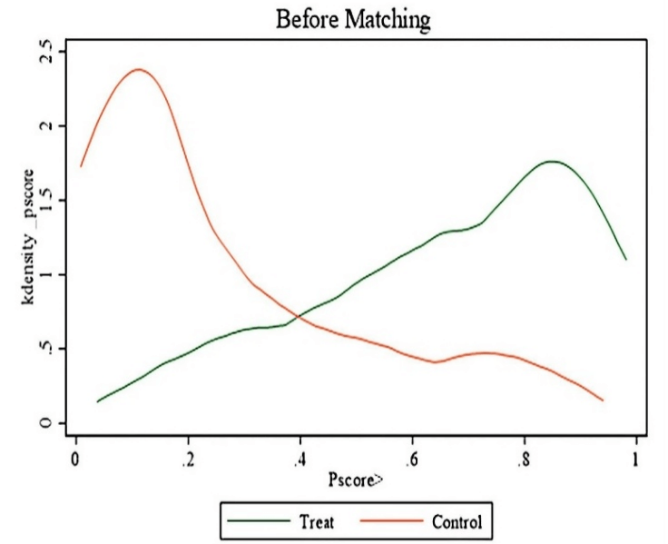
Figure 3. Kernel Density Matching Plot (Before Matching).

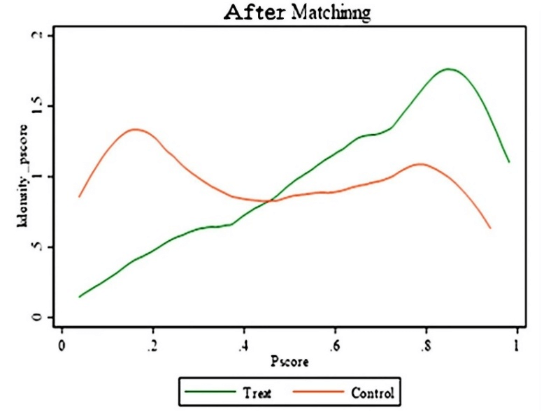
Figure 4. Kernel Density Matching Plot (After Matching).

After estimating the propensity scores, we plot their density distributions to assess the common-support region. As shown in Figures 3 and 4, the kernel-density curves of the treatment and control groups diverge markedly before matching; after matching, the two curves almost coincide, indicating a substantial improvement in overlap and confirming the quality of the propensity-score match.

Taking the nearest-neighbor specification as an example, we further validate the procedure by generating the common-support diagnostic plot using Stata 17.0 (Figure 5). The graph indicates that merely a small number of observations lie outside the overlapping region, thus the vast majority of treated households can be matched with valid controls, fulfilling the common-support assumption necessary for causal inference.

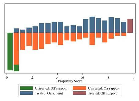
Figure 5. Test Chart for the Hypothesis of Shared Support Domains in Propensity Score Matching.

As Figure 5 illustrates, before and after matching, the vast majority of treated and control observations are located within a common support region and are densely distributed. This implies that only a small number of cases are discarded, indicating high matching quality.

The diagnostic checks affirm the robustness of the propensity-score matching: (i) each covariate’s absolute standardized bias is diminished to under 10% post-matching, meeting the balance criterion, and (ii) the propensity score kernel-density plots for both groups nearly overlap, ensuring the common-support condition with minimal sample attrition. Consequently, the PSM results are both credible and robust, suggesting that homestead withdrawal exerts a positive causal effect on the well-being of rural residents.

4.2.4. Robustness Test

To ensure robustness, we substitute the comprehensive rural well-being index with household self-reported happiness scores, which encompass factors such as income, education, employment stability, and social relationships. This single-indicator proxy directly captures subjective welfare, thereby avoiding potential noise arising from index construction and weight assignment. As shown in Table 8, the sign and significance of the estimated coefficients remain consistent with those obtained from the Logit regressions, confirming that our conclusions are insensitive to the choice of the dependent variable and reinforcing. Assessing the reliability of the earlier findings.

Table 8. Test Results using Propensity Score Matching (PSM).

Variable	Matching method	Average Treatment Effect (ATT)	Standard error	T-statistic
Rural residents Subjective well-being	Minimum Nearest Neighbor Matching	0.365	0.030	2.09
	Radius matching	0.364	0.022	1.81
	Nuclear matching	0.310	0.039	2.08
	Local linear Regression matching	0.278	0.028	1.63

In summary, the dual validation of the propensity-score matching (PSM) procedure substantiates the plausibility of the modelling assumptions. After matching, Propensity Score Matching (PSM), the standardized biases across all covariate dimensions are markedly reduced, indicating that selection bias has been effectively attenuated. The kernel-density plots of the propensity scores for the treated and control groups exhibit near-perfect overlap, confirming distributional balance. With only a few marginal observations removed, the overwhelming majority of cases remain within the common-support region, thereby safeguarding external validity. These diagnostic indicators collectively demonstrate that the PSM model achieves high goodness-of-fit and strong internal validity. In light of the empirical evidence from studies such as those conducted in Anhui Jinzhai County and Fujian Jinjiang City, Hypothesis 1—asserting that homestead withdrawal has a statistically significant and positive impact on rural residents’ well-being—has been accepted.

4.2.5. Act of Homestead Withdrawal on Various Dimensions of Rural Residents’ Well-Being

As previously outlined, the well-being indicator system for rural residents consists of four dimensions: economic status, life satisfaction, health status, and interpersonal relationships. Based on this framework, this study adopts three matching methods to examine the impact of homestead withdrawal on each dimension of rural residents’ well-being. Through these matching approaches, we measured the effects across all dimensions and found that homestead withdrawal significantly enhances rural residents’ well-being. However, the specific mechanisms underlying this effect and its impacts on individual dimensions require further verification. The results are presented in Table 9, which shows that the impact of homestead withdrawal varies across different dimensions of rural residents’ well-being, with the most significant improvement observed in economic status.

Table 9. Estimated Effects of Homestead Land Withdrawal on Various Dimensions of Rural Residents’ Well-Being.

Note: ***, **, and * indicate significance at the 1%, 5%, and 10% levels, respectively.

The terms of income, homestead withdrawal exerts a significantly positive impact on the economic well-being of rural residents. Taking the nearest neighbor matching method as an example, the economic well-being indices of the experimental group and the control group are 0.082 and 0.125, respectively. The average treatment effect (ATT) difference between the two groups is 0.012, which is highly significant at the 1% level. These findings indicate that homestead withdrawal can increase farmers’ income and improve rural residents’ economic conditions. Regarding the dimension of life satisfaction, the nearest neighbor matching method shows that the life satisfaction coefficients of the experimental group and the control group are 0.075 and 0.093, respectively. The mean treatment effect difference is 0.013, significant at the 1% level. The underlying mechanism is that homestead withdrawal improves residents’ material foundations and living environments, thereby positively affecting their life satisfaction—though this effect is subject to complex regulation by multiple subjective factors. In the dimension of health status, results from the nearest neighbor matching method reveal that the health status coefficients of the experimental group and the control group are 0.075 and 0.093, respectively. The mean treatment effect difference is 0.010, significant at the 5% level. Theoretically and empirically, homestead withdrawal may generate long-term positive health impacts by optimizing residential environments and enhancing healthcare accessibility, or interpersonal relationships. The nearest neighbor matching method indicates that the interpersonal relationship coefficients of the experimental group and the control group are 0.069 and 0.092, respectively. The mean treatment effect difference is 0.012, significant at the 10% level.

Based on the aforementioned theoretical data, Hypothesis 2 is validated.

4.3. Testing the Mediating Effect of Non-Farm Payrolls

4.3.1. Mediation Effect Model

Combined with the framework theory of rural residents’ well-being after homestead withdrawal, this paper discusses whether homestead withdrawal can improve rural residents’ well-being by affecting non-agricultural employment. Based on the mediation effect analysis method proposed by a “three-step method” regression model was established.

This study employs the mediating effect model to dissect the influence process and mechanism of independent variables on dependent variables, utilizing methods such as the Baron and Kenny stepwise approach and the Bootstrap method for assessing the significance of the mediating effect.  In examining the impact of an independent variable X on a dependent variable Y, when X influences Y via an intermediary variable M, M is identified as the mediating variable. Equations (3) to (5) delineate the relationship between variables:

 (3)

 (4)

 (5)

Among them, the coefficient c of equation (4) is the total effect of the independent variable X on the dependent variable Y. The coefficient a of equation (5) is the effect of the independent variable X on the mediating variable M. The coefficient b of equation (6) is the effect of the mediating variable M on the dependent variable Y after controlling for the influence of the independent variable X. The coefficient  is the direct effect of the independent variable X on the dependent variable Y after controlling for the influence of the mediating variable M. e₁ ~ e₃ are the regression residuals. The mediating effect is equivalent to the indirect effect, which is calculated as the product of the coefficient.

Sobel test, construct statistics:

 (6)

is the standard deviation of the  coefficient, and  is the standard deviation of the  coefficient. A significant result of statistic Z, such as Z > 1.96 at a 5% significance level, indicates that the mediating effect is significant. If the result of statistic Z is not significant, then it is clear that the mediating effect is not significant.

4.3.2. Testing for Mediating Effects

Studies employing linear regression models, such as those examining the impact of rural labor transfer on income levels and urbanization, support the use of this method to analyze the causal relationship between rural labor transfer and the well-being of rural residents. The results, as detailed in Table 10, demonstrate the significant impact of rural labor transfer on farmers’ income and economic growth.

Table 10. Mediating Effect Test.

Variable	Well-being of rural residents	Labor transfer	Well-being of rural residents
Farmers’ homesteads were withdrawn	0.054*** （0.033）	0.156*** （0.015）	0.061*** （0.126）
Labor transfer			0.398*** （0.141）

Note: The coefficients reported in the table denote marginal effects, with standard errors shown in parentheses; other variables and provincial controls have been considered.

Studies from various regions, such as Yuyang District in Jiangxi Province and Jinjiang City in Fujian Province, indicate that homestead withdrawal is positively associated with rural residents’ well-being and labor transfer to off-farm employment, with significant coefficients at the 0.1% level. Empirical evidence from studies such as indicates that off-farm transfer remains positively linked to well-being, with a coefficient of 0.389 and a significance level of p < 0.001, while the direct effect of homestead withdrawal on well-being has been observed to modestly decrease to 0.061, maintaining a significant impact. These results are significant, confirming that off-farm labor transfer serves as a partial mediator between homestead withdrawal and rural well-being.

4.3.3. Robustness Tests

When conducting path analysis for the mediating effect of non-agricultural employment, the results of the mediation test may be distorted by endogeneity between the mediating variable and the explained variable, leading to biased estimates. Therefore, selecting an appropriate robustness test method is critical. In this study, the SPSS Process macro was employed for robustness testing. This tool not only tests the significance of the mediating effect but also addresses endogeneity concerns. By generating 4,000 repeated samples via the Bootstrap method, a 95% bias-corrected confidence interval was constructed. This approach not only mitigates the issue of small sample size but also corrects for estimation bias. The Bootstrap test results for the mediation path analysis of non-agricultural employment levels are presented in Table 11.

Table 11. Bootstrap mediation effect test.

Inspection category	Path	Effect value	P > |z|	95% Confidence interval
Non-farm employment path test	The withdrawal of homesteads → non-agricultural employment → the well-being of rural residents	1.71	0.221	[0.014, 0.038]
	Homesteads are withdrawn → non-agricultural employment	2.34	0.019	[0.002, 0.022]
	Non-farm payrolls → well-being of rural residents	2.23	0.026	[0.004, 0.062]
	The withdrawal of homesteads → the well-being of rural residents	1.64	0.014	[ 0.022, 0.041]

The table shows that the 95% confidence intervals for all path tests of non-agricultural employment exclude zero, indicating a significant positive effect. This suggests that homestead withdrawal exerts a significant impact on rural residents’ well-being, with part of this impact mediated by the non-agricultural employment variable. Results of the Bootstrap mediation test are consistent with those of the stepwise regression mediation analysis, confirming the mediating role of non-agricultural employment in the relationship between homestead withdrawal and rural residents’ well-being. This verifies the robustness of the regression results regarding the non-agricultural employment pathway and validates the mediating effect of non-agricultural employment in this relationship.

5. Conclusions and Policy Implications

5.1. Research Conclusions

Based on China’s new development stage and utilizing survey data from 405 farm households in three western counties of Shandong Province, this study integrates theoretical reasoning with propensity-score matching (PSM) to ascertain the causal effect of homestead withdrawal on rural residents’ well-being. Three key findings are presented. First, relinquishing the homestead substantially enhances households’ multidimensional well-being. Second, off-farm employment serves as a crucial mediator: through reallocating labor to higher-productivity sectors, homestead exit translates land-value gains into sustained income gains and broader life satisfaction. Thirdly, PSM provides a robust tool for evaluating rural land-policy interventions, offering new evidence to refine homestead-reform design and advance the broader rural-revitalization agenda.

5.2. Policy Implications

(1)  Fine-tune policy design. Given that livelihood structures and economic capacities vary significantly among households, county-level programmes should incorporate flexible entry rules, opt-out clauses, and periodic impact reviews to enable continuous learning and real-time adjustments.

(2)  Build a differentiated compensation and rights-protection system. A dynamic model that integrates a base land price with location-specific correction coefficients can reflect regional disparities and heterogeneous functions of homesteads, ensuring both scientific rigor and perceived fairness. Transparent third-party appraisal procedures and mandatory village-level hearings should ensure farmers’ full right to information and participation, with household welfare serving as the guiding principle for every exit decision.

(3)  Enhance re-employment support and human-capital investment. For households with heavy dependency burdens, targeted vocational training, wage-subsidy contracts, and start-up micro-loans should be given priority. Local governments should simultaneously optimize the industrial layout by attracting labor-intensive agro-processing, rural e-commerce, and service enterprises, thereby creating abundant off-farm jobs to facilitate the transition from farm to non-farm work.

(4)  Strengthen the factor base for rural revitalization. Homestead reform directly relieves bottlenecks such as “no land for housing” and “no land for industrial projects” while unlocking collateral value and facilitating the free flow of labor, capital, and technology between urban and rural areas. Consolidated parcels released through the programme can be allocated to specialty agriculture, leisure farming, agritainment, or small-scale processing zones, thereby diversifying village revenue streams and enhancing homestead withdrawal within a broader strategy of industrial upgrading and shared prosperity.

(5)  While short-term cash compensation from homestead withdrawal can improve farmers’ living standards, its long-term impacts exhibit diverse, complex dynamics with heightened uncertainties. To balance immediate gains and long-term benefits, targeted policies are required to address the long-term effects of homestead withdrawal—such as refining compensation appreciation-sharing mechanisms and integrating employment support with social security systems.

CRediT Author Statement: Xue Wang: Conceptualization, Methodology, Data curation, Writing – original draft, Visualization, Investigation, Supervision, Software, Validation, and Writing – review & editing; Xiiuli Han: Writing – review & editing.

Data Availability Statement: All data used in this paper are presented within the text and are original data from this paper.

Funding: This research was funded by the National Social Science Foundation, grant number [23BJY152]; Ningxia Philosophy and Social Science Program, grant number [22NXBYJ01].

Conflicts of Interest: The authors declare no conflict of interest.

IRB Statement: Not applicable.

Informed Consent Statement: Not applicable.

Acknowledgments: The authors would like to thank National Social Science Foundation and the Ningxia Philosophy and Social Science Program for their funding support.

Abbreviations

The following abbreviations are used in this manuscript:

PSM	propensity score matching
CEM	Coarsened Exact Matching
ATT	Average Treatment effect on the Treated
SMDs	Standardized Mean Differences

References

Cao, Y., & Geng, Z. (2022). Institutional pathways on the display of homestead property value under the goal of common wealth. Dynamics of Social Sciences, (8), 28–33.

Chen, L., Song, G., & Zou, Z. (2016). Research on the exit mechanism of rural homestead land under the New Economic Normal. Rural
Economy, (7), 42–48.

Chen, M., Huang, C., Zhang, T., Guo, X., & Liu, T. (2022). Rural residential land institution reform in China: Logic and path. China Land
Science, 36(7), 26–33.
https://tdzx.jxau.edu.cn/__local/A/F7/69/68E170FBE715BAD507E44CCCFC4_449A5229_10B8AD.pdf?e=.pdf

Ding, Y. (2021). Deeply grasping the historical logic of improving people’s livelihood and well-being. Frontiers, (12), 42–49. https://doi.org/10.16619/j.cnki.rmltxsqy.2021.12.005

Gao, H., & Li, H. (2020). The change of “Two-field System” of agricultural reclamation and the reconstruction of agricultural land rights
system: A comparative perspective of state-owned and collective agricultural land. Chinese Rural Economy, 6, 37–55.
https://link.cnki.net/urlid/11.1262.F.20200622.1108.016

Han, D., Han, L., Zhang, X., & Chen, X. (2018). Study on the rural homestead buyout programs from the perspective of marketization.
Research on Agricultural Modernization, 39(1), 19–27.
https://doi.org/10.13872/j.1000-0275.2017.0118

Han, W., & Liu, L. (2021). Annual report on the development of political economy in China. China Review of Political Economy, 12(3), 53–77.

He, L., Zeng, Y., Fu, C., & Gong, C. (2020). The effect of social capital’s participating in the rejuvenation of homesteads on alleviating poverty and boosting agricultural prosperity in the perspective of rural revitalization: Based on the case and evidence of joint construction of rural houses. Journal of Management, 33(2), 11–24. https://doi.org/10.19808/j.cnki.41-1408/F.2020.02.002

Huang, G. L., Jiang, Y. Q., Liu, Z. F., Nie, M., Liu, Y., Li, J. W., Bao, Y. Y., Wang, Y. H., & Wu, J. G. (2016). Advances in human well-being research: A sustainable science perspective. Acta Ecologica Sinica, 36(23), 7519–7527.
https://doi.org/10.5846/stxb201511172326

Hu, Y. G., Yang, C. M., Dong, W. J., Wen, Q., Zhang, Y., & Lin, S. D. (2020). Farmers’ homestead exit behavior based on perceived value theory: A case of Jinzhai County in Anhui Province. Resources Science, 42(4), 685–695.
https://doi.org/10.18402/resci.2020.04.08

Jia, Y., Li, G., Zhu, X., Wang, J., & Li, Y. (2009). Study on changes in farmers’ welfare before and after concentrated housing: Based on
Amartya Sen’s Capability Approach. Issues in Agricultural Economy, (2), 30–36.

Liang, H., Luo, J., & Zhang, H. (2017). Influence of land circulation on socialized service needs for farmers’ production based on the empirical analysis of PSM model. Journal of Agrotechnical Economics, (10), 106–118.

Li, K., Yao, L., Shi, Y., Zhang, D., & Lin, Y. (2022). Estimate well-being of urban and rural residents in the Yellow River Basin and its
spatio-temporal evolution. Ecological Economics, 38(11), 222–229.
https://stjj.cbpt.cnki.net/portal/journal/portal/client/paper/69c800c11e85cca2fe0596e7ab123f8d

Luo, M., Chen, W., & Lin, Y. (2022). The effect of democratic participation on rural residents’ subjective well-being: The moderating effect of perceived social equity. Journal of South China Normal University (Social Sciences Edition), (4), 110–122.

Mao, C., Shang-Guan, C., & Feng, S. (2017). Rural residential land replacement models: Regional differences and mechanisms. Journal of Arid Land Resources and Environment, 31(10), 31–37.
https://doi.org/10.13448/j.cnki.jalre.2017.310

Niu, X., Zhou, H., Yu, Z., & Wu, G. (2022). Study on the influence of environmental perception on farmers’ homestead withdrawal willingness from the perspective of the theory of planned behavior—Based on the survey of farmers in rural suburbs in Shanghai. Chinese Journal of Agricultural Resources and Regional Planning, 43(2), 141–149.
https://link.cnki.net/urlid/11.3513.S.20211220.1438.004

Peng, J., Zeng, Y., & Fang, P. (2024). Digital economic development and rural residents’ well-being: An empirical analysis based on CFPS data. Journal of China Agricultural University, 29(5), 241–251.
https://doi.org/10.11841/j.issn.1007-4333.2024.05.22

Qiu, T., & Luo, B. (2017). Does land reallocation negatively affect rural labor migration to non-agricultural sectors? China Rural Survey, (4), 57–71. https://doi.ogr/10.20074/j.cnki.11-3586/f.2017.04.005

Qu, Y., Jiang, G., Zhang, F., & Shang, R. (2012). Models of rural residential land consolidation based on rural households’ willingness.
Transactions of the Chinese Society of Agricultural Engineering, 28(23), 232–242.

Si, R., Lu, Q., Zhang, Q., & Liang, H. (2018). Influence of land circulation on socialized service needs for farmers’ production based on the empirical analysis of PSM model. Resources Science, 40(9), 1762–1772.
https://doi.org/10.18402/resci.2018.09.07

Sun, L., & Chen, S. W. (2021). Study on the willingness, behavior and consistency of purchasing agricultural insurance: Based on the
decomposed theory of planned behaviour. Rural Economy, (11), 70–77.

Sun, P., & Zhao, K. (2020). Effect of social capital on farmers’ behavior of quitting rural residential land: A case study of 606 farmers’ samples in Jin Zhai County, Anhui Province. Journal of Nanjing Agricultural University (Social Sciences Edition), 20(5), 128–141.

Sun, X., Lin, L., & Xu, J. (2019). Farmland dependency, farmland transfer behavior, and household differentiation: An analysis based on survey data from 209 households in Fujian Province. Rural Economy, (6), 22–31.

Wang, R. (2021). The contemporary implications and significant importance of continuously enhancing people’s well-being. People’s Tribune, (9), 140–149. https://rmlt.cbpt.cnki.net/WKG/WebPublication/wkTextContent.aspx?colType=4&tp=gklb&m

Wang, Z., & Cai, Y. (2025). Scale of land expropriation, stability of non-agricultural employment, and the withdrawal of rural land contract rights in suburban areas: A case study of Wuhan City. China Land Science, 39(6), 102–112.

Yang, L., Zhu, C., Yuan, S., & Li, S. (2018). Analysis of farmers’ willingness to exit homestead land and welfare changes based on supply-side reform: A case study of Yiwu City, Zhejiang Province. China Land Science, 32(1), 35–41.
https://doi.org/10.11994/zgtdkx.20180129.121747

Yan, Z., Li, J., & Zeng, W. (2017). Analysis of homestead withdrawal intentions and policy implications: A case study of Shuangliu District, Chengdu. Rural Economy, (6), 28–34.

Yi, Q., Ma, L., & Wang, Q. (2010). Evaluation on the welfare levels of land-lost peasants based on Sen’s function and capability welfare theory. Chinca Land Science, 24(7), 41–46.
https://doi.org/10.13708/j.cnki.cn11-2640.2010.07.010

Zhang, Y., & Bao, T. (2019). An empirical study on the factors influencing farmers’ willingness to settle in city in the process of urbanization. Journal of Arid Land Resources and Environment, 33(10), 14–19.
https://doi.org/10.13448/j.cnki.jalre.2019.281

Zhou, D., & Yang, H. (2025). The impact of non-agricultural employment quality on rural household consumption. Journal of Inner Mongolia Agricultural University (Philosophy and Social Sciences Edition), 27(2), 10–17.
https://doi.org/10.16853/j.issn.1009-4458.2025.02.002

Zhou, J., Wang, W., Gong, M., & Huang, Z. ( 2020). Land transfers, occupational stratification and poverty reduction. Economic Research
Journal, 55(6), 155–171.

Zou, X., Wu, T., Xu, G., Wang, Y., Xie, M., & Li, Z. (2020). Rural social capital and household homestead withdrawal: Evidence from a sample of 522 households in Yujiang District, Jiangxi Province. China Land Science, 34(4), 26–34.