Structural Vector Autoregressive Modeling for Carbon Dioxide Emissions—Evidence from India

1. Introduction

In the intricate landscape of the contemporary global scenario, the challenge of harmonizing economic development with environmental sustainability stands as a defining imperative for nations worldwide. This challenge is further compounded by the urgent need to address the profound consequences of climate change, a global phenomenon that traverses geographical and political boundaries indiscriminately. Climate change, primarily driven by the relentless accumulation of greenhouse gases, poses an imminent and existential threat to our planet, marked by rising global temperatures, unpredictable extreme weather events, and disruptions to delicate ecosystems (Krishnan et al., 2020; Mohanty & Wadhawan, 2021). The current scientific consensus resounds unequivocally, emphasizing the imperative for immediate and concerted measures to constrain global warming’s trajectory and mitigate the multifaceted repercussions of climate change (Nathaniel et al., 2021). The crux of this global conundrum lies in the pursuit of a harmonious equilibrium—sustaining robust economic development while concurrently curbing the ominous specter of Carbon Dioxide (CO₂) emissions. Achieving this equilibrium demands a radical shift in the paradigms that underpin the conceptualization and execution of economic policies, environmental stewardship, and societal progress.

India’s per capita CO₂ emissions in 2022 stand at 1.91 t.CO₂, placing it 15th among the countries listed, ranking among the lowest on a per-person basis despite being the third-largest emitter in absolute terms globally, contributing 6.99% of total world emissions (Table 1). This contrast highlights that while individual carbon footprints in India are relatively low, the country’s sheer population size means that its total emissions remain significant on the global scale. Positioned at the forefront of the world’s fastest-growing economies, India faces a critical juncture in balancing rapid economic growth with environmental sustainability. The low per capita emissions mask the underlying challenge: a burgeoning population, rising industrialization, and expanding energy demand collectively exert pressure on carbon emissions trajectories. Amidst ambitious development goals and rising socio-economic expectations, India must navigate a complex interplay between sustaining economic growth and meeting climate commitments. The situation is further compounded by transformative shifts in climate patterns, including the increasing frequency of extreme weather events and the global rise in temperatures, underscoring the urgency of effective mitigation strategies. Consequently, understanding per capita CO₂ trends is pivotal for designing innovative policies and technological solutions that can simultaneously support economic growth, enhance energy efficiency, and reduce carbon intensity.

Table 1. Trends in country-wise CO₂ emissions.

Source: Crippa et al., 2023.

CO₂ emissions, primarily propelled by the nation’s rapid economic development, have witnessed notable trends that underscore the intricate interplay between growth and environmental sustainability. Table 1 shows that the United States, with a slightly declining yet consistent emission pattern, constitutes 12.60% of the global total in 2022. In contrast, China emerges as the predominant global emitter, accounting for a substantial 32.88% share, indicative of its rapid industrialization. Russia’s emissions display fluctuations, contributing 4.96% globally. Japan and Germany showcase relatively stable or decreasing emission levels, representing 2.81% and 1.75% of global emissions, respectively. Notably, India exhibits a noteworthy increase in emissions, although it maintains a comparatively lower per capita footprint. Contributing 6.99% to global emissions in 2022, India’s trajectory reflects the complexities of balancing economic growth and environmental concerns. This rise in emissions, while lower on a per capita basis, is indicative of the intricate challenges faced in balancing economic growth and environmental considerations. Factors like growing population, intensified industrial activities, and heightened energy demands play a role in shaping India’s emissions trajectory, emphasizing the imperative for the formulation and implementation of sustainable development strategies.

As one of the world’s fastest-growing economies, India faces the dual challenge of sustaining economic growth while addressing the rise in CO₂ emissions, an inherent aspect of its developmental trajectory. The increasing frequency of extreme weather events and rising global temperatures further emphasize the urgency of mitigating the environmental impacts of this growth. India’s contribution to the global carbon footprint, although shaped by its unique local dynamics, resonates on an international scale, underlining the need for innovative approaches that transcend traditional economic metrics and recognize the deep interconnections between ecological sustainability and long-term economic resilience. Achieving this delicate balance is crucial, not only for India’s future but for global efforts to secure a sustainable and resilient future for all nations.

The existing literature on India’s CO₂ emissions highlights the tension between rapid economic expansion and its environmental consequences, yet there remain significant research gaps, particularly regarding sector-specific emissions. Key industries such as energy, transportation, and agriculture, which form the backbone of India’s economy, contribute disproportionately to its carbon footprint, but their distinct roles in shaping emission trends are often overlooked. Additionally, the effects of India’s policy shifts—such as its increasing focus on renewable energy, technological innovation, and environmental regulations—on emission trajectories have not been fully explored. A nuanced understanding of how these factors interact with macroeconomic variables over time is vital for the development of effective and targeted policy interventions. Furthermore, the complex relationship between India’s demographic dynamics—urbanization, population growth, and industrialization—and CO₂ emissions demands more granular analysis. These demographic shifts play a critical role in shaping energy demand and carbon output, yet their full implications are not adequately addressed in current studies. The interaction of these variables, alongside environmental factors such as forest cover, offers a rich area for further research to better understand the drivers of emissions and the strategies needed to mitigate them.

To address these gaps, the present study employs Structural Vector Autoregressive (SVAR) modeling, a sophisticated analytical tool that allows for the identification of dynamic cause-and-effect relationships between key variables influencing CO₂ emissions. By incorporating variables such as Gross Fixed Capital Formation (GFCF), Gross National Product (GNP), Population (POP), and Forest Cover (FC), the SVAR model captures the complex interdependencies driving emissions in India. GFCF, as a measure of investment in infrastructure and industrial processes, directly influences energy consumption, a major source of CO₂ emissions. GNP, representing the total economic output, often correlates with higher emissions as growth intensifies industrial activities. Population size, with its impact on energy demand, urbanization, and consumption patterns, is another critical factor, while forest cover, which acts as a carbon sink, plays a crucial role in balancing emissions. By applying the SVAR model to these variables, the study offers valuable insights into the long-term effects of policy interventions, such as the National Action Plan on Climate Change (NAPCC), renewable energy adoption, and industrial reforms, on India’s emission trajectory. The model also accounts for external shocks—such as fluctuations in global oil prices or climate-related disasters—that can influence CO₂ emissions, thus providing a more comprehensive understanding of the forces at play. India’s experience serves as a compelling case study with far-reaching global implications. As the world grapples with the challenge of harmonizing economic growth and environmental sustainability, India’s struggle reflects the broader global effort to reconcile these competing priorities. This study, by delving into the intricacies of India’s emissions dynamics, not only addresses the country’s unique challenges but also offers a valuable blueprint for other nations facing similar dilemmas. The findings from this research contribute to the global discourse on sustainable development, providing actionable insights that can help shape the future path toward a resilient and ecologically balanced global economy.

2. Background

Review of relationships between economic growth, fixed capital investments, population growth, and CO₂ emissions has garnered researchers’ attention since the 1990s because of increasing recognition of the interconnectedness between economic development and environmental sustainability. The most relevant studies are illustrated in Table 2.

 

Table 2. Categorization of Empirical Studies on CO₂ Emissions.

The reviewed literature reveals several key research gaps and inconsistencies. First, the relationship between economic growth and CO₂ emissions remains inconclusive, with some studies (Ayobamiji & Kalmaz, 2020; Sbia et al., 2014) reporting a positive association, while others (Bozkurt & Akan, 2014) find a negative one—indicating that the Environmental Kuznets Curve (EKC) hypothesis may not be universally applicable. Furthermore, many existing studies (e.g., Ozturk, 2010; Payne, 2010) rely on traditional VAR or cointegration approaches that do not account for structural shocks, limiting their causal interpretability and policy relevance. Another gap is the limited use of the Structural VAR (SVAR) model in the Indian context—despite the country’s rapid economic growth and evolving energy landscape, only Tiwari (2011) has applied this framework. In addition, factors such as gross fixed capital formation, industrial restructuring, and energy intensity remain underexplored, though they critically influence emission patterns. The role of renewable energy also appears ambiguous, as Silva et al. (2012) identified short-term economic trade-offs, whereas Tiwari (2011) observed clear emission-reducing effects, underscoring the need for context-specific dynamic modeling.

Against this background, the present study contributes to the literature by employing an SVAR model to capture structural shocks and dynamic interactions among economic growth, energy use, and CO₂ emissions in India. By imposing identification restrictions, the study enhances the interpretability of causal mechanisms and provides a more accurate understanding of policy transmission effects. This structural approach not only fills a methodological gap in the Indian context but also yields policy-relevant insights into how targeted interventions in the energy and industrial sectors can influence carbon emissions, thereby offering a more robust framework for sustainable economic and environmental planning.

3. Materials and Methods

In this paper, the SVAR model incorporates GNP, GFCF, POP, and FC to capture the key drivers of CO₂ emissions in India through three channels—scale, composition, and technique. GNP reflects the scale of economic activity; GFCF represents investment and industrial structure; POP measures demographic pressure; and FC serves as a proxy for natural carbon sequestration. Together, these variables mirror the main policy levers influencing emissions. The SVAR framework is used because it allows identification of structural shocks—such as investment, growth, or land-use changes—and traces their dynamic impacts on CO₂ through impulse responses and variance decomposition. This approach offers policy-relevant insights by distinguishing short-run and long-run causal effects that conventional VAR models cannot capture. It is important to acknowledge the limitations in the selection of determinants, particularly the risk of omitted-variable bias. Key factors such as total energy consumption, energy mix (coal, gas, renewables), energy intensity, technological progress, trade openness, urbanization, and explicit policy instruments (e.g., taxes, subsidies, regulations) are not included and could potentially confound the estimated structural responses. Additionally, measurement challenges—including differing data frequencies, revisions in forest cover and CO₂ series, and uncertainties in land-use emission accounting—along with sample-size constraints, may reduce the precision and reliability of the inferences drawn from the analysis (Buckle et al., 2002).

3.1. Data Sources

For the analysis, we used CO₂ emissions (m. tonnes), real GNP (million US$), GFCF (million US$), POP (million), and FC (million ha). The secondary data are collected from multiple sources, viz., World Bank Indicators (CO₂ emissions); FAOSTAT and Agricultural Statistics at a Glance, Government of India, for other selected variables during 1990 to 2022. For the purpose of analysis, all variables are transformed into logarithms as it minimizes the fluctuations in the data series (Apergis & Payne, 2010; Tiwari, 2010).

3.2. Structural Vector-Autoregression

In this study, the Ng-Perron unit root test, recently developed by Ng and Perron (2001), was chosen to assess the stationarity of time series. Ng and Perron sought to address the limitations of ADF and PP tests by introducing a set of four test statistics (Yıldırım et al., 2015). These tests include the MZa (Modified Zivot-Andrews); MZt (Modified Zivot-Andrews with a structural break at an unknown time); MSB (test which is the modified version of the Bhargava test); and MPT (Modified versions of Augmented Dickey-Fuller-Generalized Least Squares [ADF-GLS] test). For the Ng and Perron (2001) test, the fundamental hypothesis sets a unit root for the MZa and MZt tests, and stationarity for the MSB and MPT tests. The determination of the lag length to be incorporated in our analysis is based on the Akaike Information Criteria (AIC) due to its superior performance in small sample sizes (Liew, 2004).

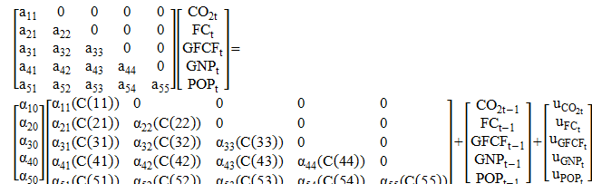
The SVAR methodology meticulously examines the intricate interactions among all variables, and its constraints are grounded in economic theory or disclose information regarding the dynamic properties of the investigated economy (Narayan et al., 2008). Consequently, this model proves invaluable for predicting the ramifications of precise policy interventions or significant transformations in the economy, as exemplified in scenarios involving alterations in CO₂ emissions (Buckle et al., 2002; Narayan et al., 2008). The following SVAR is formulated:

 (1)

The generalized form can be represented as:

 (2)

In the above generalized form,  is a  vector of endogenous variables,  is a  matrix of lag coefficients to be estimated on  lag,  is a  vector of white noise innovation processes representing the structural shocks.  is a matrix that reflects the contemporaneous relationship among endogenous variables.

Now considering the study, here vector  includes five variables: CO₂ emissions, FC, GFCF, GNP, and POP. The system is represented as shown below:

(3)

(4)

(5)

 (6)

 (7)

The matrix form of the above system is given as:

 (8)

To derive the reduced form VAR, multiply both sides of Equation (1) by ; we get:

 (9)

Multiplying a matrix with its inverse gives an identity matrix, i.e., , where  is the identity matrix. Thus, the above equation can be written as:

 (10)

where vector  depends on lag of itself and the forecast error . The matrix  here also indicates the forecast errors of VAR,  and the structural shocks  i.e., . In reduced form VAR,  is the linear makeup of .

Structural VAR is basically a conceptually constructed framework and is non-observable (Jena et al., 2023). Thus, it cannot be computed directly. As we have time series or a history of variables, we use these to estimate the VAR. Following that, the regression of each variable is run against its lag and the lag of other variables included in the VAR. Hence, we get the coefficient  and the forecast error . Starting from the reduced form VAR estimation, our goal is to get the structural model that isolates the purely exogenous shocks and responds to the variables of interest. To do this, we would need to get matrix , or more precisely, we need to restrict matrix . Get  and multiply the reduced form VAR by  to get the structural model, shocks, and contemporaneous channelization among the variables (Auclert et al., 2021; Cravino et al., 2020).

 (11)

After getting the structural model, we impose restrictions on contemporaneous relationships among endogenous variables of the structural model. This is what identification entails. Identification means imposing restrictions on matrix  based on economic intuition. From the calculated coefficients, the SVAR with both short-run restriction is presented as follows:

 (12)

Similarly, SVAR with imposing long-run restriction is given as:

 (13)

In the computation of SVAR, we must impose restrictions on the parameter matrices (Garratt et al., 1998). These restrictions can take the form of either contemporaneous restrictions on the parameter matrices of A₀ and B, where A₀ and B are the (K × K) matrices indicating instantaneous relationship relations of variables in X_t and ε_t, respectively, or long-run restrictions on the total effects of structural shocks to identify the structural parameters. In this paper, we employ both short-run and long-run restrictions methods (Blanchard & Quah, 1989). For example, in the long-run restrictions model, A₀ is set as an identity matrix, i.e., A₀ = I_K. These restrictions are based on long-run restrictions imposed on the cumulative impulse response function. In total, K(K − 1)/2 restrictions are imposed on the lower triangular matrix, where some of the structural shocks do not have contemporaneous impacts on the other variables. The variables are ordered as follows: CO₂ emissions, FC, GFCF, GNP, and POP. For the Recursive Short-Run Impulse Response (S triangular) and Recursive Long-Run Impulse Response (F triangular) models, the same principles are applied, but with variations in the imposition of restrictions based on specific characteristics of each model (Blanchard & Quah, 1989; Love & Zicchino, 2006; Sims, 1980). The conceptual framework of SVAR is illustrated in Figure 1.

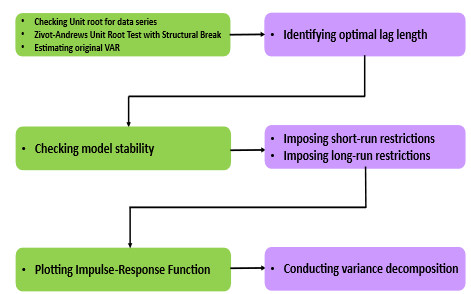
Figure 1. Conceptual framework of SVAR.

4. Results

4.1. Unit Root Tests and Structural Break

The unit root tests (Table 3), employing both Ng and Perron (2001) and Zivot and Andrew methodologies (Adewole et al., 2020), contribute valuable insights into the stationarity and structural properties of the variables (Mollick, 2009). In their level form, CO₂ emissions, FC, GFCF, GNP, and POP exhibit non-stationary behavior, as evidenced by consistently smaller calculated statistical values for the MZa and MZt tests compared to critical values. Conversely, the MSB and MPT tests show statistical values surpassing critical values, further affirming non-stationarity. However, the transformation through differencing renders the variables stationary, with first differences demonstrating the absence of a unit root at both 1 and 5% significance levels. The Zivot and Andrew test reveals unit roots in the levels of all variables, but structural breaks (Table 4), identified as A (Intercept), B (Trend), and C (Trend and Intercept), signify shifts in their properties at specific years. These findings collectively provide a robust foundation for justifying the application of a Structural VAR model, as it accommodates the stationary nature post-differencing and captures the dynamic relationships amidst structural shifts in the economic system.

Table 3. Ng- Perron Unit Root Test Results.

Variable	MZa	MZt	MSB	MPT
Level form
CO2 emissions	−2.2801	−0.8010	0.3523	9.0793
Critical Value	−5.7078	−1.6206	0.2753	4.4521
FC	−1.1402	−0.3530	0.3099	10.0861
Critical Value	−5.7026	−1.6213	0.2751	4.4566
GFCF	0.3669	0.6210	1.6930	161.8241
Critical Value	−5.7026	−1.6222	0.2753	4.4524
GNP	−5.0039	−1.4327	0.2864	5.2639
Critical Value	−5.7018	−1.6225	0.2754	4.4536
POP	−1.6475	−0.6890	0.4189	37.9777
Critical Value	−14.2045	−2.6207	0.1853	6.6771
First difference form
CO2 emissions	−31.2232**	−24.5354**	0.0242**	0.0514**
Critical Value	−13.8432	−2.5991	0.1746	1.7927
FC	−34.4600**	−14.7234**	0.1043**	0.7341**
Critical Value	−13.8337	−2.5898	0.1748	1.7968
GFCF	−16.7291**	−3.8958*	0.1736*	1.5224*
Critical Value	−13.8762	−2.6044	0.1748	1.7966
GNP	−11.8807*	−3.1095*	0.2151*	2.9499*
Critical Value	−8.1374	−1.9924	0.2345	3.1915
POP	−7.0997*	−2.7722*	0.2509*	3.8971*
Critical Value	−5.7228	−1.6269	0.2758	4.4828

Note: ** & * - shows the absence of unit roots at 1% and 5% significance levels, respectively.

Table 4. Results of Zivot and Andrew unit root test.

Variables	tcal	Structural break down	Structural break year	Order of Integration
CO2 emissions	−7.9371**	A	2009	I(1)
FC	−3.5391**	A	2001	I(1)
GFCF	−4.0714**	A	2004	I(1)
	−4.1409*	B	2011
	−3.9354**	C	2004
GNP	−3.5352*	A	2005	I(1)
	−2.5050*	B	2012
POP	−0.4519*	B	2017	I(1)

Note: Break location: A = Intercept, B = Trend, C = Trend and Intercept;

** & * - shows the absence of unit roots at 1% and 5% significance levels, respectively.

 

4.2. Lag Selection Criteria

Table 5 shows the outcome of the lag selection criteria. The result indicates that the majority of lag selection criteria—such as FPE, AIC, SC, and HQ—suggest an optimal lag length of 4 (Liew, 2004). This convergence across multiple criteria enhances confidence in the selection of lag 4, affirming its suitability for the cointegration test as well as estimating the SVAR.

Table 5. VAR lag length criteria.

Lag	LogL	LR	FPE	AIC	SC	HQ
0	368.0973	NA	3.75e−18	−25.93552	−25.69763	−25.86280
1	643.9278	433.4480	6.42e−26	−43.85199	−42.42463	−43.41563
2	692.8481	59.40312*	1.41e−26	−45.56058	−42.94375	−44.76058
3	731.3286	32.98331	9.38e−27	−46.52347	−42.71717	−45.35985
4	798.6051	33.63826	1.95e−27*	−49.54322*	−44.54746*	−48.01597*

Note: *indicates lag order selected by the criterion; LR - sequential modified LR test statistic (each test at 5% level; FPE: Final prediction error; AIC: Akaike information criterion; SC: Schwarz information criterion; HQ: Hannan-Quinn information criterion.

4.3. Johansen Cointegration Test

Findings from Table 6 highlight both trace and maximum eigenvalue tests to ascertain the presence of a long-run relationship among the analyzed variables. The trace test assesses various hypotheses concerning the number of cointegrating equations, providing compelling evidence in favor of cointegration. At the 0.05 significance level, the trace statistic exceeds the critical values for all scenarios considered, strongly indicating the existence of a cointegrating relationship. Similarly, the maximum eigenvalue test supports these findings, displaying statistical significance for the same scenarios. Consistently, both tests suggest the presence of four cointegrating equations, bolstering the robustness of this conclusion. These results establish a fundamental groundwork for subsequent SVAR analysis, confirming the interconnectedness of variables in the long run.

Table 6. Results of Johansen Cointegration test.

Unrestricted Cointegration Rank Test (Trace)
Hypothesized No. of CE(s)	Eigenvalue	Trace Statistic	0.05 Critical Value	Prob.**
None *	0.974171	217.2628	69.81889	0.0000
At most 1 *	0.840717	114.8873	47.85613	0.0000
At most 2 *	0.699031	63.44932	29.79707	0.0000
At most 3 *	0.654845	29.82838	15.49471	0.0002
At most 4	0.001536	0.043037	3.841465	0.8356
Unrestricted Cointegration Rank Test (Maximum Eigenvalue)
Hypothesized No. of CE(s)	Eigenvalue	Max-Eigen Statistic	0.05 Critical Value	Prob.**
None *	0.974171	102.3755	33.87687	0.0000
At most 1 *	0.840717	51.43798	27.58434	0.0000
At most 2 *	0.699031	33.62094	21.13162	0.0006
At most 3 *	0.654845	29.78534	14.26460	0.0001
At most 4	0.001536	0.043037	3.841465	0.8356

Note: Trace test indicates 4 cointegrating eqn(s) at the 0.05 level.

     Max-eigenvalue test indicates 4 cointegrating eqn(s) at the 0.05 level.

4.4. Stability Test

We conducted a stability test, assessing the stationary properties of variables using the AR root table (Table 7) and the corresponding graph (Figure 2). The findings showed that all the roots of the characteristic polynomial exhibit moduli less than one. The accompanying graph illustrates that all the unit circles lie inside the circle, indicative of the VAR model’s variance and covariance stationarity, meeting the necessary stationary conditions. This observation underscores the stability of the model, affirming its suitability for analyzing the dynamic relationships among variables over time. The consistent moduli below one signify that the system is not prone to explosive or divergent behavior, enhancing the reliability of the SVAR results derived from this model.

Table 7. Results of the AR root table.

Root	Modulus
−0.242359 + 0.781007i	0.814177
−0.168252 – 0.821575i	0.802511
0.808526	0.808526
0.992080	0.992080
0.954869 − 0.265886i	0.991196
0.954869 + 0.265886i	0.991196
0.594543 − 0.728428i	0.940260
0.594543 + 0.728428i	0.940260
0.331748 + 0.844647i	0.907461
0.331748 − 0.844647i	0.907461
−0.779670 − 0.449947i	0.900187
−0.779670 + 0.449947i	0.900187
−0.525968 − 0.712170i	0.885341
−0.525968 + 0.712170i	0.885341
0.592544 + 0.464048i	0.752629
0.592544 − 0.464048i	0.752629
−0.647900	0.647900
−0.070119 + 0.622368i	0.626306
−0.070119 − 0.622368i	0.626306
0.073044	0.073044

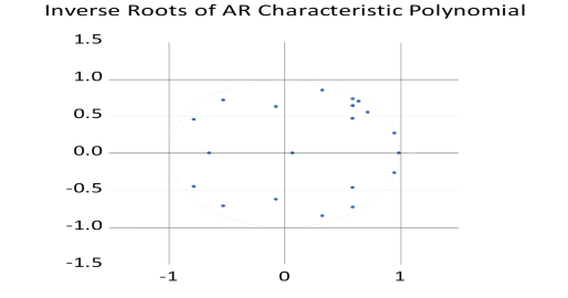
Figure 2. AR Root Graphic.

4.5. Test for Normality of Residuals

The analysis of VAR residuals (Table 8) for normality reveals encouraging results, with skewness values for all components near zero and non-significant chi-square tests, indicating a lack of substantial skewness in the data. Similarly, kurtosis results across all components exhibit non-significance, and the joint test does not reach significance either, suggesting that the tails of the distribution do not deviate significantly from normality. The Jarque-Bera test, considering both skewness and kurtosis, further supports these findings, indicating no individual or joint significance. Collectively, these tests provide robust evidence that the VAR residuals adhere well to multivariate normality.

 

Table 8. Skewness, Kurtosis, and Jarque-Bera Test for Normality of VAR residuals.

Component	Skewness	Chi-sq	df	Prob.*
1	0.0039	0.0001	1	0.9921
2	0.3667	0.8457	1	0.3578
3	0.5609	1.8988	1	0.1682
4	0.1057	0.0724	1	0.7879
5	0.1135	0.0835	1	0.7727
Joint		2.9004	5	0.7153
Component	Kurtosis	Chi-sq	df	Prob.
1	3.1919	1.6642	1	0.1970
2	2.3801	0.3551	1	0.5512
3	3.0921	0.0467	1	0.8289
4	3.0223	0.9967	1	0.3172
5	3.0252	0.9907	1	0.3196
Joint		8.7315	5	0.1203
Component	Jarque-Bera	df	Prob.
1	1.6643	2	0.4351
2	1.2008	2	0.5486
3	1.9455	2	0.3781
4	5.7472	2	0.0565
5	1.0741	2	0.5845
Joint	11.6320	10	0.3104

Note: *Approximate p-values do not account for coefficient estimation.

4.6. Test for Autocorrelation of Residuals

The VAR Residual Serial Correlation LM Test assesses whether the residuals from the estimated VAR model are serially correlated across different time lags (Table 9). The first part of the test examines serial correlation at individual lags, while the second part evaluates the joint absence of correlation across multiple lags. In this study, the adjusted test results indicate that all probability values exceed the 5% significance level, leading to the acceptance of the null hypothesis of no serial correlation. This confirms that the residuals are independently distributed, implying that the VAR model is correctly specified and the dynamic relationships among the variables are appropriately captured without systematic errors in the error structure. These independently distributed residuals are crucial for generating valid Impulse Response Functions (IRFs) in a VAR model. They ensure that each shock represents a unique, exogenous disturbance, free from overlap with past errors. This independence allows the IRF to accurately trace the pure dynamic response of one variable to another over time. Consequently, it enhances the credibility of causal interpretations and the reliability of policy inferences derived from the model.

Table 9. VAR Residual Serial Correlation LM Tests.

Null hypothesis: No serial correlation at lag h
Lag	LRE* stat	df	Prob.	Rao F-stat	df	Prob.
1	18.642	25	0.812	NA	(25, NA)	NA
2	22.754	25	0.644	NA	(25, NA)	NA
3	20.389	25	0.727	NA	(25, NA)	NA
4	24.117	25	0.508	NA	(25, NA)	NA
Null hypothesis: No serial correlation at lags 1 to h
Lag	LRE* stat	df	Prob.	Rao F-stat	df	Prob.
1	18.642	25	0.812	NA	(25, NA)	NA
2	38.416	50	0.875	NA	(50, NA)	NA
3	54.229	75	0.929	NA	(75, NA)	NA
4	69.357	100	0.943	NA	(100, NA)	NA

 

4.7. SVAR for Short-Run and Long-Run Restrictions

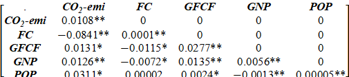
The short-term SVAR estimations (Buckle et al., 2002) reveal the immediate dynamics among CO₂ emissions, FC, GFCF, GNP, and POP (Table 10). A positive and statistically significant self-impact of CO₂ emissions (0.0108**) indicates that current emission levels influence future emissions even in the short term, reflecting the persistence of carbon-intensive practices. Economically, this suggests that emission reductions cannot occur instantaneously; short-term policy interventions must be complemented by sustained structural changes to industrial processes and energy use (Bernanke, 1986; Blanchard & Watson, 1986; Sims, 1986).

Table 10. Results of Structural VAR Estimate on Short-run pattern.

Variables		Coefficient	Std. Error	z-Statistic	Prob.
	C(1)	0.0108**	0.0014	7.4833	0.0000
	C(2)	−0.0841**	0.0277	−3.0399	0.0024
	C(3)	0.0131*	0.0059	2.1976	0.0280
	C(4)	0.0126**	0.0035	3.5960	0.0003
	C(5)	0.0311*	0.0142	2.1929	0.0283
	C(6)	0.0001**	0.0000	7.4833	0.0000
	C(7)	−0.0115*	0.0055	−2.1121	0.0347
	C(8)	−0.0072*	0.0029	−2.4693	0.0135
	C(9)	0.00002	0.00001	1.6578	0.0974
	C(10)	0.0277**	0.0037	7.4833	0.0000
	C(11)	0.0135**	0.0021	6.4669	0.0000
	C(12)	0.0024*	0.0011	2.2964	0.0217
	C(13)	0.0056**	0.0007	7.4833	0.0000
	C(14)	−0.0013**	0.0004	−3.3387	0.0008
	C(15)	0.00005**	0.00001	7.4833	0.0000
R2 = 0.79**; Adj R2 = 0.72**
Akaike Information Criterion (AIC): –4.87
Bayesian Information Criterion (BIC): –4.11

Note: ** and * - Significance at 1 and 5% levels respectively.

The negative immediate effect of FC (−0.0841**) demonstrates that short-term increases in forested area can reduce CO₂ emissions. Although the magnitude may appear moderate numerically, at the national scale even small increments in forest cover translate into substantial carbon sequestration, emphasizing the short-term mitigation potential of afforestation, reforestation, and forest conservation programs.

GFCF (0.0131*) shows a positive immediate effect on CO₂ emissions, indicating that short-term expansions in capital investment, especially in industrial and infrastructure sectors, quickly translate into higher emissions. This underscores the environmental cost of rapid capital deployment unless investments are directed toward low-carbon or energy-efficient technologies. Similarly, GNP (0.0126**) positively affects CO₂ emissions, reflecting the short-term responsiveness of emissions to economic output. The magnitude suggests that even modest increases in economic activity can immediately elevate carbon output, highlighting the challenge of balancing short-term growth with environmental sustainability.

Finally, POP growth (0.0311*) contributes positively to short-term CO₂ emissions. The relatively larger magnitude compared to GFCF and GNP indicates that demographic pressures quickly amplify energy demand, consumption, and industrial activities, thus increasing emissions. This finding aligns with classical economic interpretations that population expansion drives short-run energy consumption patterns and environmental stress (Bernanke, 1986; Blanchard & Watson, 1986; Sims, 1986).

These short-run coefficients quantify the relative influence of each determinant on immediate emissions. Forest cover acts as a mitigating factor, while population, economic output, and investment accelerate emissions even in the short term. These results highlight the need for targeted short-term policies—such as afforestation incentives, energy-efficient investment programs, and demand-side management—to moderate emissions while structural and technological transitions take effect. The Adjusted R² confirms that the SVAR model is statistically sound, with a high explanatory power and efficient specification. Further, the low AIC and BIC values indicate optimal lag selection and model parsimony, supporting the credibility of the structural dynamics and impulse response analysis derived from the estimated coefficients.

 (14)

Under the long-run restrictions of the SVAR model, a clearer picture of the persistent dynamics among CO₂ emissions and its determinants emerges (Table 11). The self-impact of CO₂ emissions (0.5413**) indicates strong persistence, implying that past emission levels continue to drive future emissions. Economically, this suggests that once carbon-intensive practices are embedded in industrial and energy systems, they tend to persist, necessitating deliberate structural interventions—such as decarbonizing energy infrastructure or retrofitting industrial processes—to break this inertia.

Table 11. Results of Structural VAR Estimate on Long-run pattern.

Variables		Coefficient	Std. Error	z-Statistic	Prob.
	C(1)	0.5413**	0.0730	7.4109	0.0000
	C(2)	−0.0387**	0.0052	−7.4078	0.0024
	C(3)	0.6293*	0.0850	7.4035	0.0280
	C(4)	0.5477**	0.0739	7.4079	0.0003
	C(5)	0.1663*	0.0224	7.4104	0.0283
	C(6)	0.0007**	0.0001	7.4793	0.0000
	C(7)	−0.0153*	0.0032	−4.7573	0.0347
	C(8)	−0.0101*	0.0016	−6.1502	0.0135
	C(9)	0.0011	0.0002	6.1278	0.0974
	C(10)	0.0131**	0.0018	7.4823	0.0000
	C(11)	0.0035**	0.0008	4.3156	0.0000
	C(12)	0.0067*	0.0102	0.6562	0.0217
	C(13)	0.0035**	0.0005	7.4861	0.0000
	C(14)	−0.0002**	0.0001	−2.4021	0.0008
	C(15)	0.0005**	0.0001	7.4769	0.0000
R2 = 0.81**; Adj R2 = 0.77**
Akaike Information Criterion (AIC): –5.12
Bayesian Information Criterion (BIC): –4.42

Note: ** and * - Significance at 1 and 5% levels respectively.

The negative effect of FC (−0.0387**), though modest in magnitude, reflects the cumulative carbon sequestration benefits of increased forest area. While the coefficient appears small numerically, even slight increases in forest cover can offset emissions significantly at the national scale, particularly given India’s large land area. Economically, this underscores the long-term value of afforestation, reforestation, and forest conservation policies as a cost-effective carbon mitigation strategy.

GFCF (0.6293*) exhibits the largest long-run positive impact among the variables, indicating that investments, particularly in infrastructure and industrial capacity, substantially elevate CO₂ emissions. This highlights the trade-off between investment-led growth and environmental sustainability, emphasizing the urgency of integrating green technologies, renewable energy infrastructure, and energy-efficient capital into development planning.

The effect of GNP (0.5477**) on CO₂ emissions also remains large and positive, reflecting that economic expansion continues to be heavily reliant on carbon-intensive sectors and fossil fuels. The magnitude implies that sustained growth without structural transformation in the energy and industrial sectors will exacerbate emission pressures, reinforcing the importance of policies promoting low-carbon economic growth.

Finally, POP growth (0.1663*) contributes positively but at a smaller magnitude compared to investment and output. This indicates that while demographic expansion increases aggregate energy demand and consumption, its effect on emissions is less pronounced per unit change than structural or economic factors. Economically, this implies that energy efficiency measures, urban planning, and sustainable consumption patterns can partially offset the emission pressures of population growth.

Taken together, the long-run coefficients quantify the relative contributions of each factor to persistent CO₂ emissions. Investment and economic growth are the largest drivers, suggesting that structural and technological shifts are critical to achieving sustainable development. Forest cover plays a mitigating role, and population growth, though smaller in magnitude, still requires targeted policies for energy conservation and efficiency. These insights provide actionable guidance for policymakers aiming to balance economic development with long-term environmental sustainability. The high R² and adjusted R² indicate that the model explains a substantial portion of the variation in the data, while the low AIC and BIC values reflect its efficiency and suitability. Together, these diagnostics confirm that the long-run SVAR model robustly captures the structural relationships among CO₂ emissions, GFCF, GNP, POP, and FC, providing a reliable basis for deriving meaningful long-term policy insights.

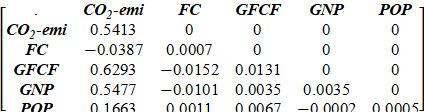 (15)

4.8. IRF of CO₂ Emissions

The IRFs (Table 12; Figures 3; Figure 4) analyze the dynamic responses of CO₂ emissions to one-standard-deviation shocks in FC, GFCF, GNP, and POP. In Figure 3, CO₂ emissions show a brief increase after a FC shock, peaking in the first period and fading by the third, suggesting a temporary emission rise from land-use changes or forestry activities (e.g., land preparation, biomass burning) before sequestration benefits emerge. The 95% confidence intervals reflect uncertainty, but the effect is short-lived. CO₂ emissions response to GFCF shock remains near zero, indicating minimal short-term impact, possibly due to green technology adoption or lagged effects. Conversely, GNP and POP shocks drive steady increases in CO₂ emissions, with effects strengthening after the fifth and second periods, respectively, reflecting sustained emission pressures from economic growth and population demand. The initial FC response may reflect VAR framework issues, such as Cholesky ordering assuming exogeneity, capturing correlated shocks (e.g., land-use policies) rather than sequestration. Measurement challenges (e.g., aggregating forest types, lags in carbon uptake) and initial emissions from afforestation (e.g., machinery, soil release) may also contribute (Sims, 1980). Socio-economically, this could indicate transitional emissions in developing economies from infrastructure-linked forest programs, with long-term sequestration potentially offsetting these, supporting sustainability goals (Ewing et al., 2007; Robalo & Salvado, 2008). Integrated policies balancing forest management, economic, and demographic strategies are thus essential.

Table 12. IRF of CO₂ emissions to innovations (Cholesky ordering).

Period	FC	GFCF	GNP	POP
1	0.0068	0.0000	0.0000	0.0000
2	0.0047	0.0001	0.0006	0.0004
3	0.0039	0.0011	0.0007	0.0004
4	0.0022	0.0024	0.0017	0.0008
5	0.0012	0.0039	0.0020	0.0017
6	0.0001	0.0046	0.0037	0.0026
7	−0.0014	0.0057	0.0048	0.0033
8	−0.0026	0.0061	0.0069	0.0054
9	−0.0038	0.0076	0.0095	0.0061
10	−0.0045	0.0091	0.0112	0.0098

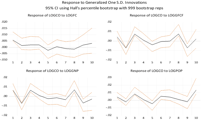
Figure 3. Structural Response (IRF) of CO₂.

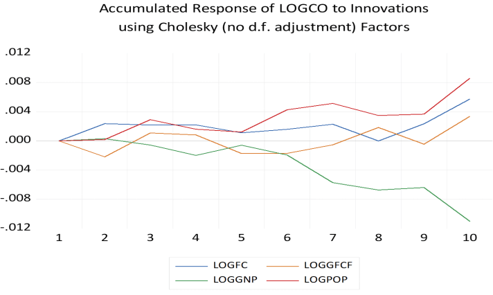
Figure 4. Accumulated Response (IRF) of CO₂.

Figure 4 shows CO₂ emissions accumulated response to FC starting slightly negative, dipping mid-period, then rising modestly, suggesting initial emission costs are offset by sequestration over time. GFCF response stabilizes near zero, reinforcing its short-term neutrality. GNP and POP exhibit cumulative increases, with notable rises after the fifth and sixth periods, respectively, highlighting their long-term emission drivers. The Cholesky ordering may amplify initial FC effects due to data or ordering assumptions, aligning with ecological models of maturing carbon sinks (Ewing et al., 2007; Sims, 1980).

4.9. Structural Variance Decomposition to CO₂ Emissions

While IRF offers insights into the impact of variable changes on others, quantifying the magnitude or degree of these effects requires the variance decomposition method. This method delves into the percentage differences in the dependent series attributable to shocks from various variables (Ahmad et al., 2015; Ewing et al., 2007; Hassan et al., 2016; Saidu et al., 2018). The variance decomposition estimates over a 10-year projection period (Table 13) distinguishes between short-term and long-term effects. The first to fifth periods are classified as short-term, and the sixth to tenth periods as long-term. This comprehensive analysis allows us to identify the key drivers of predicted variations in the system, shedding light on the dynamic interplay of different factors over various time horizons. The findings showed that in the first period, the entire variance in CO₂ emissions is attributed to its own shock (100%), indicating that the initial impact on carbon emissions is predominantly driven by internal factors. However, as we progress, the influence of CO₂ emissions diminishes, and other variables come into play. By the second period, the shock in FC becomes a significant contributor (12.43%), signaling the short-term influence of forest cover changes on CO₂ emissions. In the subsequent periods, GFCF, GNP, and POP gradually gain importance, with GNP and POP becoming the primary drivers in later periods. This decomposition underscores the evolving nature of the determinants of CO₂ emissions, highlighting the shifting roles of different factors over time. The increasing contributions of economic growth (GNP) and population growth (POP) suggest the enduring impact of these variables on carbon emissions in the long run.

Table 13. Structural variance decomposition of CO₂.

Period	S.E.	CO2 emissions	FC	GFCF	GNP	POP
1	0.0108	100.0000	0.0000	0.0000	0.0000	0.0000
2	0.0134	76.6917	12.4308	10.6005	0.1989	0.0780
3	0.0166	57.1342	8.2215	22.6267	1.2030	10.8147
4	0.0174	56.0764	7.4599	20.6272	3.7952	12.0413
5	0.0185	49.7821	7.9749	25.7831	5.6453	10.8147
6	0.0197	43.9693	7.2785	22.7435	6.8498	19.1590
7	0.0217	39.5637	6.4034	19.9038	17.7270	16.4020
8	0.0235	37.7880	9.2798	21.0575	15.8852	15.9896
9	0.0247	36.7040	11.9924	22.4362	14.4140	14.4534
10	0.0303	26.8225	12.9622	21.2542	18.8871	20.0741

The above findings are stable, as indicated by all eigenvalues lying within the circle, and hence underscore their reliability for informed forecasting and policy recommendations. In tune with sustainable development goals, India must strategically enhance economic growth, focusing on sectors like manufacturing, agriculture, and energy utilization. Integration of innovation, science, and technological advancements into the developmental agenda becomes imperative. The above findings resonate the need for a balanced approach to economic growth and environmental sustainability. India, as a rapidly developing nation, faces the challenge of accommodating robust economic expansion while mitigating carbon emissions. Furthermore, the study highlights the distorting impact of GFCF on CO₂ emissions. So, the Foreign Direct Investment (FDI) activities should strictly adhere to standardized environmental regulations. As India evolves, its financial sector should prioritize environmental quality by directing banking activities toward supporting renewable energy and low-carbon ventures. The role of GFCF as a determinant factor of environmental quality in early development, particularly due to emissions from multinational corporations, holds relevance for India’s industrialization trajectory. India, in attracting FDI, needs to adopt policies that rigorously evaluate the environmental implications of multinational corporations’ activities before granting permits. This cautious approach is vital to ensure balance between economic growth and environmental protection in mitigating the detrimental effects of FDI on climate (Jakada et al., 2022).

4.10. Granger Causality Test

The analysis in Table 14, employing the lag length determined by the AIC of the VAR model, elucidates significant long-run influences of all variables on CO₂. In all the pairs, the rejection of the null hypothesis for both directions indicates bidirectional causality among selected variables. The bidirectional causality between FC and CO₂ emissions indicates a dynamic and reciprocal relationship. The rejection of the null hypothesis that FC does not Granger cause CO₂ underscores the significant impact of changes in forest cover on subsequent variations in CO₂ emissions, aligning with the recognized role of forests as carbon sinks. Conversely, the rejection of the null hypothesis that CO₂ does not Granger cause FC highlights the influence of past CO₂ emissions on future forest cover patterns, emphasizing the interconnected nature of these environmental variables. This bidirectional causality underscores the importance of incorporating forest management in climate change mitigation strategies. Similarly, the bidirectional causality observed between GFCF and CO₂ emissions implies a reciprocal influence over the long run.  This reciprocal influence implies that as investment in fixed capital increases or decreases, it affects the levels of CO₂ emissions. Conversely, changes in CO₂ emissions also play a role in shaping future patterns of GFCF. This bidirectional causality underscores the interconnected nature of economic activities and environmental outcomes, highlighting that economic development and carbon emissions are mutually influencing factors over the long term. The understanding of this reciprocal relationship is crucial for policymakers and environmental planners to develop comprehensive strategies that consider the environmental implications of economic activities and vice versa. The bidirectional relationships in GNP and POP pairs emphasize the interconnectedness between economic growth, population size, and CO₂ emissions. This suggests that economic activities and population dynamics not only influence carbon emissions but are also influenced by past emissions, illustrating the intricate web of interactions shaping the long-term trajectories of these variables.

Table 14. Granger causality test.

Null Hypothesis	Obs	F-Statistic	Prob.
FC does not Granger Cause CO2	28	3.8327	0.0190
CO2 does not Granger Cause FC		4.5657	0.0094
GFCF does not Granger Cause CO2	28	5.2351	0.0051
CO2 does not Granger Cause GFCF		3.1849	0.0368
GNP does not Granger Cause CO2	28	3.6747	0.0235
CO2 does not Granger Cause GNP		3.0662	0.0412
POP does not Granger Cause CO2	28	3.4509	0.0279
CO2 does not Granger Cause POP		9.3631	0.0002

5. Conclusions

In the complex landscape of India’s rapid economic growth, the challenge of curbing CO₂ emissions becomes a critical focal point, influenced by demographic and socio-economic dynamics unique to the nation. Amidst ambitious development goals and escalating environmental concerns, the interplay of GFCF, GNP, POP, and FC emerges as a linchpin. This study, employing the SVAR model, delves into the intricate relationships among these variables to unravel patterns that can inform sustainable environmental management strategies. Unlike the conventional VAR approach prevalent in extant literature, SVAR transcends limitations by adeptly capturing the nuanced structural relationships among variables without necessitating restrictive identification measures, as often mandated by traditional methods. This methodological innovation not only enhances the scholarly landscape but also fills a notable void in the understanding of the Indian economy.

The findings underscore the urgency of addressing the environmental repercussions of India’s growth, especially considering transformative shifts in climate patterns and the surge in CO₂ emissions. India’s notable increase in emissions, contributing 6.99% to the global total in 2022, reflects the complexities of balancing economic growth and environmental concerns. As India positions itself at the forefront of global economies, the study becomes a crucial tool for policymakers and economic forecasters. The SVAR model reveals both short-term and long-term insights. The short-term analysis reveals a notable immediate impact of a one-unit shock to CO₂ emissions, emphasizing the persistence in emissions and posing challenges to rapid carbon reduction. FC exhibits a short-term role in decreasing emissions, underscoring its potential as a carbon sink. Short-term increases in capital formation (GFCF) and economic output (GNP) contribute to heightened CO₂ emissions, highlighting the intricate link between economic activities and carbon output. Population growth (POP) shows a positive immediate effect on emissions. In the long run, CO₂ emissions exhibit a sustained pattern, emphasizing the challenges in transitioning away from carbon-intensive activities. Increased forest cover contributes to long-term emission reduction, while the positive effects of GFCF and GNP underscore the dilemma of achieving economic growth without increased carbon output. Population growth continues to influence long-term CO₂ emissions, highlighting the importance of both sustainable population management and energy-efficient strategies. The IRF reveals the short-term dynamics following shocks in forest cover, capital formation, economic output, and population growth. Economic growth and population growth contribute to elevated emissions, emphasizing the need for comprehensive policies addressing forest conservation, sustainable economic practices, and population management. The Structural Variance Decomposition further quantifies the contributions of different shocks to the predicted fluctuations in CO₂ emissions, showing the enduring impact of economic and population growth in the long run. Further, bidirectional causality is evident across various pairs, emphasizing the dynamic and reciprocal relationships among selected variables. Recognizing these bidirectional relationships is crucial for policymakers and environmental planners to formulate comprehensive strategies that balance economic development with environmental sustainability. This further underscores the complexity of achieving sustainable development and underscores the need for integrated, holistic approaches to address environmental challenges.

In conclusion, this study underscores the imperative of adopting a harmonized approach to economic growth and environmental sustainability in India. While acknowledging the pivotal role of economic growth in the country’s development, the findings emphasize the simultaneous need for strategic interventions to curtail carbon emissions. Key focal points for intervention include:

·  Both policymakers and enterprises should adopt concrete and targeted measures to balance economic growth with environmental sustainability. Emission reduction targets are crucial, including clear, time-bound national and sectoral CO₂ goals aligned with India’s climate commitments, such as achieving net-zero emissions by 2070. These targets should be integrated into state-level development plans to ensure coordinated implementation across regions.

·  Renewable energy development must be accelerated, with expanded deployment of solar, wind, and bioenergy technologies. Strengthening grid infrastructure, storage solutions, and incentivizing distributed generation and off-grid renewables can reduce dependence on fossil fuels and support a cleaner energy transition.

·  Green investment and technological innovation are essential to decouple growth from carbon emissions. Fiscal incentives, subsidies, and tax benefits can encourage enterprises to adopt low-carbon production processes, energy-efficient infrastructure, and sustainable capital formation. Additionally, research and development in carbon capture, storage, and sustainable manufacturing should be prioritized.

·  Addressing demographic pressures through sustainable population and urban planning is also critical. Energy-efficient urban designs, compact cities, expanded public transport, and building codes for energy conservation can help manage the environmental impact of population growth.

·  To ensure economic development remains sustainable, balancing FDI with environmental protection is necessary. Environmental compliance standards for foreign direct investment should be established, while green FDI projects adopting renewable energy, energy efficiency, or low-carbon technologies should receive preferential treatment.

·  Introducing carbon pricing mechanisms, such as carbon taxes or emissions trading systems, can further strengthen India’s mitigation framework. Carbon taxation would internalize the environmental cost of pollution, incentivize cleaner production, and generate revenue that can be reinvested in renewable energy, reforestation, and green infrastructure projects.

·  Finally, forest conservation and afforestation play a vital role in mitigating emissions. Strengthened policies for forest protection, reforestation, and afforestation, combined with incentives for private sector participation and carbon credit schemes, can maximize carbon sequestration and enhance environmental resilience.

By implementing these integrated strategies, India can sustain economic growth while effectively mitigating CO₂ emissions. The study underscores the importance of holistic, multi-sectoral approaches that combine energy policy, investment planning, population management, and environmental regulation to achieve long-term sustainability goals.

CRediT Author Statement: This is a single-author paper, and the author takes sole responsibility for all aspects of the work, including concept development, study design, data analysis, manuscript drafting, and revision.

Data Availability Statement: The data are available from the corresponding author upon reasonable request.

Funding: This research received no external funding.

Conflicts of Interest: The author declares no conflict of interest.

IRB Statement: Not applicable.

Informed Consent Statement: Not applicable.

Acknowledgments: Not applicable.

Abbreviations

The following abbreviations are used in this manuscript:

CO2-emi	Carbon Dioxide emissions
GFCF	Gross Fixed Capital Formation
GNP	Gross National Product
POP	Population
FC	Forest Cover
FDI	Foreign Direct Investment

References

Adewole, A. I., Bodunwa, O. K., & Akinyanju, M. M. (2020). Structural vector autoregressive modeling of some factors that affect the
economic growth in Nigeria. Science World Journal, 15(2), 11–15.
https://www.ajol.info/index.php/swj/article/view/202938

Ahmad, A. U., Abdullah, A., Abdullahi, A. T., & Muhammad, U. A. (2015). Stock market returns and macroeconomic variables in Nigeria: Testing for dynamic linkages with a structural break. Scholars Journal of Economics, Business and Management, 2(8A), 816–828.
https://www.researchgate.net/publication/288616691

Antonakakis, N., Chatziantoniou, I., & Filis, G. (2017). Energy consumption, CO₂ emissions, and economic growth: An ethical dilemma.
Renewable and Sustainable Energy Reviews, 68, 808–824. https://doi.org/10.1016/j.rser.2016.09.105

Apergis, N., & Payne, J. E. (2010). Renewable energy consumption and economic growth: Evidence from a panel of OECD countries. Energy Policy, 38(1), 656–660. https://doi.org/10.1016/j.enpol.2009.09.002

Aqeel, A., & Butt, M. S. (2001). The relationship between energy consumption and economic growth in Pakistan. Asia-Pacific Development Journal, 8(2), 101–110. https://www.unescap.org/sites/default/files/apdj-8-2-ResNote-1-AQEEL.pdf

Auclert, A., Malmberg, H., Martenet, F., & Rognlie, M. (2021). Demographics, wealth, and global imbalances in the twenty-first century.
National Bureau of Economic Research. https://doi.org/10.3386/w29161

Ayobamiji, A. A., & Kalmaz, D. B. (2020). Reinvestigating the determinants of environmental degradation in Nigeria. International Journal of Economic Policy in Emerging Economies, 13(1). https://doi.org/10.1504/IJEPEE.2020.106680

Bernanke, B. S. (1986). Alternative explanations of the money-income correlation. Carnegie-Rochester Conference Series on Public Policy, 25, 49–99. https://doi.org/10.1016/0167-2231(86)90037-0

Blanchard, O. J., & Quah, D. (1989). The dynamic effects of aggregate demand and supply disturbances. American Economic Review, 79(4), 655–673. https://www.jstor.org/stable/1827924

Blanchard, O. J., & Watson, M.W. (1986). Are business cycles all alike? In R. J. Gordon (Ed.), The American business cycle: Continuity and change (pp. 123–180). University of Chicago Press. http://www.nber.org/chapters/c10021

Bowden, N., & Payne, J. E. (2009). The causal relationship between U.S. energy consumption and real output: A disaggregated analysis. Journal of Policy Modeling, 31(2), 180–188. https://doi.org/10.1016/j.jpolmod.2008.09.001

Bozkurt, C., & Akan, Y. (2014). Economic growth, CO2 emissions and energy consumption: The Turkish case. International Journal of Energy Economics and Policy, 4(3), 484–494. https://www.econjournals.com/index.php/ijeep/article/view/878

Buckle, R. A., Kim, K., Kirkham, H., McLellan, N., & Sharma, J. (2002). A structural VAR model of the New Zealand business cycle. New
Zealand Government, The Treasury. https://hdl.handle.net/10419/205501

Cheng, B. S., & Andrews, D. R. (1998). Energy and economic activity in the United States: Evidence from 1900 to 1945. Energy Sources, 20(1), 25–33. https://doi.org/10.1080/00908319808970040

Cravino, J., Lan, T., & Levchenko, A. A. (2020). Price stickiness along the income distribution and the effects of monetary policy. Journal of Monetary Economics, 110, 19–32. https://doi.org/10.1016/j.jmoneco.2018.12.001

Crippa, M., Guizzardi, D., Pagani, F., Banja, M., Muntean, M., Schaaf, E., Becker, W., Monforti-Ferrario, F., Quadrelli, R., Risquez Martin, A., Taghavi-Moharamli, P., Köykkä, J., Grassi, G., Rossi, S., Brandao De Melo, J., Oom, D., Branco, A., San-Miguel, J., & Vignati, E. (2023). GHG emissions of all world countries – 2023. Publications Office of the European Union.
https://doi.org/10.2760/953322

Erbaycal, E. (2008). Disaggregated energy consumption and economic growth: Evidence from Turkey. International Research Journal of
Finance and Economics, (20), 1–8. https://www.sid.ir/paper/608791/en

Ewing, B. T., Sari, R., & Soytas, U. (2007). Disaggregate energy consumption and industrial output in the United States. Energy Policy, 35(2), 1274–1281. https://doi.org/10.1016/j.enpol.2006.03.012

Ferreira, P., Soares, I., & Araújo, M. (2005). Liberalisation, consumption heterogeneity and the dynamics of energy prices. Energy Policy, 33(17), 2244–2255. https://doi.org/10.1016/j.enpol.2004.05.003

Garratt, A., Lee, K., Pesaran, M. H., & Shin, Y. (1998). A long-run structural macroeconometric model of the UK. The Economic Journal, 113(487), 412–455. https://doi.org/10.1111/1468-0297.00131

Halicioglu, F. (2009). An econometric study of CO₂ emissions, energy consumption, income, and foreign trade in Turkey. Energy Policy, 37(3), 1156–1164. https://doi.org/10.1016/j.enpol.2008.11.012

Hassan, A., Babafemi, O. D., & Jakada, A. H. (2016). Financial market development and economic growth in Nigeria: Evidence from VECM approach. International Journal of Applied Economics Studies, 4(3), 1–13.
https://www.researchgate.net/publication/321772982

Jakada, A. H., Mahmood, S., Ahmad, A. U., Muhammad, I. G., Danmaraya, I. A., & Yahaya, N. S. (2022). Driving forces of CO2 emissions based on impulse response function and variance decomposition: A case of the main African countries. Environmental Health
Engineering and Management Journal, 9(3), 223–232. https://doi.org/10.34172/EHEM.2022.23

Jalil, A., & Mahmud, S. F. (2009). Environment Kuznets curve for CO₂ emissions: A cointegration analysis for China. Energy Policy, 37(12), 5167–5172. https://doi.org/10.1016/j.enpol.2009.07.044

Jena, P. K., Sharma, R., Dehury, T., & Nayak, S. (2023). Impact of monetary policy transmission on the demographic in India: A structural VAR approach. Asian Economics Letters, 4(3). https://doi.org/10.46557/001c.77815

Krishnan, R., Sanjay, J., Gnanaseelan, C., Mujumdar, M., Kulkarni, A., & Chakraborty, S. (Eds.). (2020). Assessment of climate change over the
Indian region: A Report of the Ministry of Earth Sciences (MoES), Government of India. Springer.
https://doi.org/10.1007/978-981-15-4327-2

Li, Y. (2023). An empirical study on the factors influencing carbon emissions in Heilongjiang Province based on VAR model. E3S Web of
Conferences, 406, 03033. https://doi.org/10.1051/e3sconf/202340603033

Liew, V. K.-S. (2004). Which lag length selection criteria should we employ? Economics Bulletin, 3(33), 1–9. https://www.researchgate.net/publication/4827253

Love, I., & Zicchino, L. (2006). Financial development and dynamic investment behavior: Evidence from panel VAR. The Quarterly Review of Economics and Finance, 46(2), 190–210. https://doi.org/10.1016/j.qref.2005.11.007

Mohanty, A., & Wadhawan, S. (2021). Mapping India’s climate vulnerability – A district level assessment. Council on Energy, Environment and Water. https://images.hindustantimes.com/images/app-images/2021/11/ceew-study-on-climate-change-vulnerability-index-and-district-level-risk-assessment.pdf

Mollick, A. V. (2009). Employment responses of skilled and unskilled workers at Mexican maquiladoras: The effects of external factors. World Development, 37(7), 1285–1296. https://doi.org/10.1016/j.worlddev.2008.10.008

Narayan, P. K., Narayan, S., & Prasad, A. (2008). A structural VAR analysis of electricity consumption and real GDP: Evidence from the G7 countries. Energy Policy, 36(7), 2765–2769. https://doi.org/10.1016/j.enpol.2008.02.027

Narayan, P. K., & Prasad, A. (2007). Electricity consumption–real GDP causality nexus: Evidence from a bootstrapped causality test for 30 OECD countries. Energy Policy, 36(2), 910–918. https://doi.org/10.1016/j.enpol.2007.10.017

Nathaniel, S., Barua, S., Hussain, H., & Adeleye, N. (2021). The determinants and interrelationship of carbon emissions and economic growth in African economies: Fresh insights from static and dynamic models. Journal of Public Affairs, 21(1), e2141. https://doi.org/10.1002/pa.2141

Ng, S., & Perron, P. (2001). Lag length selection and the construction of unit root tests with good size and power. Econometrica, 69(6), 1519–1554. https://doi.org/10.1111/1468-0262.00256

Oryani, B., Koo, Y., & Rezania, S. (2020). Structural vector autoregressive approach to evaluate the impact of electricity generation mix on economic growth and CO₂ emissions in Iran. Energies, 13(16), 4268.
https://doi.org/10.3390/en13164268

Ozturk, I. (2010). A literature survey on energy–growth nexus. Energy Policy, 38(1), 340–349.
https://doi.org/10.1016/j.enpol.2009.09.024

Payne, J. E. (2010). A survey of the electricity consumption-growth literature. Applied Energy, 87(3), 723–731.
https://doi.org/10.1016/j.apenergy.2009.06.034

Ramos-Martín, J., & Ortega-Cerdà, M. (2003, February 12–15). Non-linear relationship between energy intensity and economic growth. ESEE Conference Frontiers 2, Tenerife, Spain.
https://www.researchgate.net/profile/Jesus-Ramos-Martin-2/publication/228424347

Robalo, P. B., & Salvado, J. C. (2008). Oil price shocks and the Portuguese economy since the 1970s. FEUNL Working Paper Series, No. 529. https://doi.org/10.2139/ssrn.1091172

Saidu, B. M., Ahmed, B. A., & Jakada, A. H. (2018). The determinants of long run economic growth in Nigeria. Asian Economic and Financial Review, 8(1), 1–8. https://doi.org/10.18488/journal.aefr.2018.81.1.7

Sbia, R., Shahbaz, M., & Hamdi, H. (2014). A contribution of foreign direct investment, clean energy, trade openness, carbon emissions and economic growth to energy demand in UAE. Economic Modelling, 36, 191–197.
https://doi.org/10.1016/j.econmod.2013.09.047

Silva, S., Soares, I., & Pinho, C. (2012). The impact of renewable energy sources on economic growth and CO2 emissions - a SVAR approach. European Research Studies Journal, 15(4), 133–144.
https://doi.org/10.35808/ersj/374

Sims, C. A. (1980). Comparison of interwar and postwar business cycles: Monetarism reconsidered. American Economic Review, 70(2), 250–257. https://www.nber.org/system/files/working_papers/w0430/w0430.pdf

Sims, C. A. (1986). Are forecasting models usable for policy analysis? Quarterly Review, 10(1), 2–16.
http://www.minneapolisfed.org/research/QR/QR1011.pdf

Stern, D. I. (1993). Energy and economic growth in the USA: A multivariate approach. Energy Economics, 15(2), 137–150. https://doi.org/10.1016/0140-9883(93)90033-N

Tiwari, A. K. (2010). Globalization and wage inequality: A revisit of empirical evidences with new approach. Journal of Asian Business
Management, 2(1), 173–187.

Tiwari, A. K. (2011). A structural VAR analysis of renewable energy consumption, real GDP and CO₂ emissions: Evidence from India.
Economics Bulletin, 31(2), 1793–1806. http://www.accessecon.com/Pubs/EB/2011/Volume31/EB-11-V31-I2-P164.pdf

Yıldırım, S., Ertuğrul, H. M., & Soytaş, U. (2015). Türkiye’de aylık istihdam serisinin durağanlığı: Geleneksel, yapısal kırılmalı ve mevsimsel birim kök test uygulamaları [Stationarity properties of monthly employment in Turkey: Conventional, structural break and seasonal unit root tests]. Anadolu Üniversitesi Sosyal Bilimler Dergisi, 15(4), 91–102.